
Lecture 10: More on Machine Learning#
In this lecture, we will continue our introduction to machine learning discussion to ensemble methods. In addition, we will also discuss unsupervised learning models, particularly, Principal Component Analysis and Clustering.
Ensemble Methods#
Techniques that combine multiple models to create a more accurate predictive model.
Several types of ensemble models:
Bagging: Multiple models are trained independently on a random subset of training data. Predictions are then averaged (regression) or voted (classification) to produce a final prediction.
Boosting: Build models sequentially with each model focusing on correcting the errors in previous ones.
Stacking: Involves training multiple models and then using another model to combine outputs in the best possible way.
Examples of Ensemble Methods#
Random Forest: A versatile ensemble method that builds multiple decision trees using random subsets of data and features, and averages their predictions to improve accuracy and control overfitting.
LightGBM: A highly efficient gradient boosting framework that uses histogram-based algorithms and leaf-wise growth to speed up training and improve performance on large datasets.
XGBoost: An optimized gradient boosting library that implements a regularized version of gradient boosting, focusing on speed and performance, particularly in terms of handling sparse data and large-scale problems.
ExtraTrees: An ensemble method similar to Random Forest, but it builds trees with more randomness by selecting cut-points for splits randomly, which often leads to more diverse trees and sometimes better generalization.
Decision Tree Classifier Explained#
A Decision Tree Classifier is a type of supervised learning algorithm used for both classification and regression tasks. It works by splitting the data into subsets based on the most significant attribute that maximizes the distinction between different classes.
Tree Building Algorithm#
In general, the tree-building algorithms use the following steps:
Evaluate the set of features and splits and pick a ”best” feature-and-split.
Add a node to the tree that represents the feature-split.
For each descendant, work with the matching data and either:
If the targets are similar enough, return a predicted target.
If not, return to step 1 and repeat.
How it Works#
Root Node: The algorithm starts at the root node, which contains the entire dataset.
Splitting: The data is split into subsets based on an attribute that best separates the classes. This decision is made using metrics like Gini Impurity or Information Gain (Entropy):
Gini Impurity: Measures the probability of a randomly chosen element being misclassified if it was randomly labeled according to the distribution of labels in the subset.
\(\text{Gini}(D) = 1 - \sum_{i=1}^{n} p_i^2\)
Information Gain: Measures the reduction in entropy when a dataset is split on an attribute.
\(\text{Information Gain} = \text{Entropy before} - \text{Entropy after}\)
Nodes and Branches: After the first split, the process is recursively applied to each subset, creating nodes (decision points) and branches (possible outcomes).
Leaf Nodes: The splitting process continues until the data cannot be split further (all samples in a node belong to a single class) or until it reaches a predetermined stopping criterion (e.g., maximum depth or minimum number of samples). The final nodes, called leaf nodes, represent the class label.
Key Characteristics#
Interpretability: Decision trees are easy to understand and interpret. The decisions can be visualized as a tree-like structure.
No Need for Feature Scaling: Unlike other algorithms, decision trees do not require feature scaling or normalization.
Prone to Overfitting: Decision trees can easily overfit the data, especially if they grow too deep. Pruning techniques or setting a maximum depth can help mitigate this.
Advantages#
Simple to understand and interpret.
Can handle both numerical and categorical data.
Requires little data preprocessing.
Disadvantages#
Prone to overfitting, particularly with deep trees.
Small variations in the data can lead to entirely different splits, making the model unstable.
Less effective for very complex datasets without ensemble methods like Random Forest.
Example Use Cases#
Customer Segmentation: Classifying customers into different segments based on purchasing behavior.
Medical Diagnosis: Classifying patients based on symptoms and test results.
Loan Approval: Deciding whether to approve a loan based on applicant attributes.
In the example below, we will see how a basic decision tree classfier works in classfiying the three different species of the Iris flowers we discussed in past lectures.
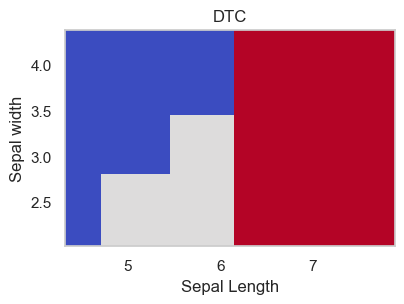
# First, let's import the necessary libraries including the ones for machine learning, data manipulation, and visualization. We will also suppress any FutureWarnings for cleaner output, but keep in mind that this is generally not recommended for production code.

#%% Ensemble Machine Learning Model

# Initialisation
import pandas as pd
from IPython.display import display

import warnings
# Suppress the FutureWarning. This is bad practice and should not be used in regular coding.
warnings.simplefilter(action='ignore', category=FutureWarning)

import matplotlib.pyplot as plt
import matplotlib.image as mpimg

import numpy as np

import seaborn as sns

import zipfile, os

from PIL import Image


# Light GBM
# To install: >>> conda install lightgbm
import lightgbm as lgb

# XGBoost
# To install: >>> conda install xgboost
import xgboost

# skopt (scikit-optimize)
# To install: >>> conda install -c conda-forge scikit-optimize
from skopt import BayesSearchCV
from skopt.space import Real, Categorical, Integer

# sklearn
from sklearn import model_selection
from sklearn.model_selection import train_test_split, RepeatedKFold
from sklearn import datasets, neighbors, metrics, ensemble
from sklearn import tree
from sklearn.linear_model import LogisticRegression
from sklearn import naive_bayes
from sklearn.neural_network import MLPClassifier

# pickle for ML model saving an dloading
from pickle import dump, load
---------------------------------------------------------------------------
ModuleNotFoundError                       Traceback (most recent call last)
Cell In[1], line 27
     22 from PIL import Image
     25 # Light GBM
     26 # To install: >>> conda install lightgbm
---> 27 import lightgbm as lgb
     29 # XGBoost
     30 # To install: >>> conda install xgboost
     31 import xgboost

ModuleNotFoundError: No module named 'lightgbm'
# We are going to use sklearn's Iris dataset for this example

# Load the iris data set from sklearn's datasets
iris = datasets.load_iris()

# Create a dataframe iris_df to contain feature names and values
# There are 4 features (sepal length and width; petal length and width)
iris_df = pd.DataFrame(iris.data, columns=iris.feature_names)

# Add in the target (y) variable into the iris_df dataframe
# There are 3 Iris species: setosa (target = 0), versicolor (target = 1) and virginica (target = 2)
iris_df['target'] = iris.target

# Create a label for the species for plotting
# Dictionary for mapping
dictionary = {i: str(iris.target_names[i]) for i in range(len(iris.target_names))}

# Applying the mapping
iris_df['species'] = iris_df['target'].map(dictionary)

display(pd.concat([iris_df.head(3),iris_df.tail(3)]))
from sklearn import tree
#%% Tree Classifier model for the Iris data

tree_classifiers = {'DTC' : tree.DecisionTreeClassifier(max_depth=3)}

# the punch line is to predict for a large grid of data points
# http://scikit-learn.org/stable/auto_examples/neighbors
# /plot_classification.html
def plot_boundary(ax, data, tgt, model, dims, grid_step = .01):
    # grab a 2D view of the data and get limits
    twoD = data[:, list(dims)]
    min_x1, min_x2 = np.min(twoD, axis=0) + 2 * grid_step
    max_x1, max_x2 = np.max(twoD, axis=0) - grid_step

    # make a grid of points and predict at them
    xs, ys = np.mgrid[min_x1:max_x1:grid_step,
    min_x2:max_x2:grid_step]
    grid_points = np.c_[xs.ravel(), ys.ravel()]

    # warning: non-cv fit
    preds = model.fit(twoD, tgt).predict(grid_points).reshape(xs.shape)

    # plot the predictions at the grid points
    ax.pcolormesh(xs,ys,preds,cmap=plt.cm.coolwarm) # 0 Blue; 1 Grey; 2 Red
    ax.set_xlim(min_x1, max_x1)#-grid_step)
    ax.set_ylim(min_x2, max_x2)#-grid_step)

fig, ax = plt.subplots(1,1,figsize=(4,3))

for name, mod in tree_classifiers.items():
    # plot_boundary only uses specified columns
    # [0,1] [sepal len/width] to predict and graph
    plot_boundary(ax, iris.data, iris.target, mod, [0,1])
    ax.set_title(name)
    plt.tight_layout()
    ax.set_xlabel('Sepal Length')
    ax.set_ylabel('Sepal width')

# initialise Decision Tree Model
dtc = tree.DecisionTreeClassifier()
# Fit decision tree model on Iris data (use 3-fold Cross-Validation)
# and compute prediction accuracy
print("3-fold CV Decision Tree accuracy on Iris data ")
model_selection.cross_val_score(dtc,
                                iris.data,
                                iris.target,
                                cv=3,
                                scoring='accuracy')
Visualising the Decision Tree#
While clustering (unsupervised learning) finds hidden patterns in unlabeled data, a Decision Tree is a form of supervised learning. Here, we know the historical outcomes (the labels), and the algorithm acts like a strategic flowchart, learning the optimal “if-then” rules to separate the data into those known categories.
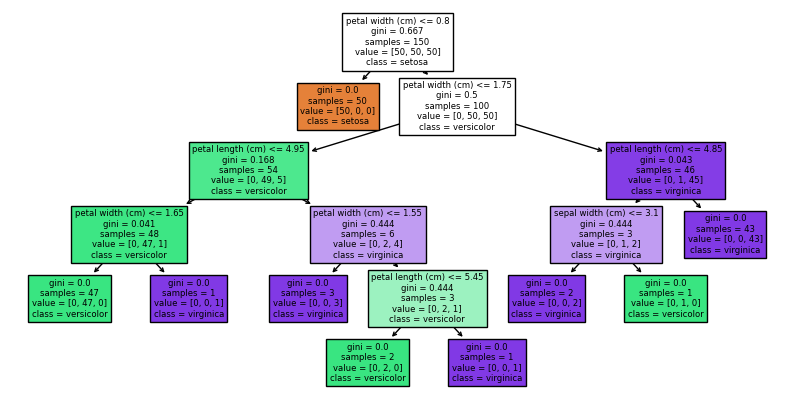
The image above visualizes a model trained on the famous Iris dataset to classify three species of flowers: Setosa, Versicolor, and Virginica.
This example of decision tree model is highly valuable because it is a “White-Box” model. Unlike deep neural networks, we can see exactly how the algorithm is making its decisions.
Let’s break down how to read this visualization:
1. The Anatomy of a Decision Node#
Look at the very top box (the Root Node). It contains all our data before any splits are made. Every box (node) contains five key pieces of information:
The Rule (e.g.,
petal width (cm) <= 0.8): This is the condition the algorithm has chosen to split the data. It scans all features and finds the single rule that best separates the classes.gini(Impurity Score): Gini impurity measures how “mixed” the data is in this box. A score of \(0.0\) means perfect purity (only one class is present). A higher number means the node is a mix of different classes. Mathematically, it is calculated as \(Gini = 1 - \sum p_i^2\), where \(p_i\) is the probability of a sample belonging to class \(i\). The algorithm’s entire goal is to minimize this Gini score with every split.samples: The total number of observations (data points) sitting in this node. The root starts with 150.value(e.g.,[50, 50, 50]): The breakdown of those samples by class. In the root, we have a perfectly balanced dataset: 50 Setosa, 50 Versicolor, and 50 Virginica.class: The majority prediction. If the model had to guess right now, this is what it would predict.
2. Tracing the Logic (Following the Branches)#
When a condition is met (True), we move down to the Left. When it is not met (False), we move to the Right.
The Easy Win (Orange Node): Notice the first split on the left. If a flower’s petal width is \(\le 0.8\) cm, the model identifies it with 100% certainty as Setosa. The Gini drops to \(0.0\), the node turns solid orange, and the model stops splitting here. This is called a Leaf Node.
The Tougher Decisions: If the petal width is \(> 0.8\) cm (moving right), the data is perfectly mixed between Versicolor and Virginica (
value = [0, 50, 50]). The algorithm must generate new rules (likepetal width <= 1.75andpetal length <= 4.95) to keep sifting the data.
3. Key Takeaways#
Color Coding Indicates Confidence: The background colors (Orange, Green, Purple) represent the predicted class. The darker the shade, the purer the node (lower Gini impurity), meaning the model is highly confident in its prediction. Lighter shades mean the model is still dealing with mixed data.
Feature Importance: By looking at the tree, we can tell which variables drive business outcomes. Notice that
petal widthandpetal lengthare heavily used to make decisions, whilesepalmeasurements barely appear. In a business context (e.g., predicting customer churn), this tells you exactly which KPIs actually matter.The Danger of Overfitting: Look at the very bottom branches of the tree. The model is creating highly specific rules just to separate nodes with only 1 or 2 samples. In machine learning, this is called overfitting. The model is memorizing the training data rather than learning general patterns. In a real business application, we would “prune” this tree (force it to stop growing earlier) so it performs better on new, unseen data.
dtc.fit(iris.data,iris.target)
plt.figure(figsize=(10,5))
tree.plot_tree(dtc, filled=True, feature_names=iris.feature_names, class_names=['setosa','versicolor','virginica'])
plt.show()
More Advanced Ensemble Methods#
Random Forest: A versatile ensemble method that builds multiple decision trees using random subsets of data and features, and averages their predictions to improve accuracy and control overfitting.
LightGBM: A highly efficient gradient boosting framework that uses histogram-based algorithms and leaf-wise growth to speed up training and improve performance on large datasets.
XGBoost: An optimized gradient boosting library that implements a regularized version of gradient boosting, focusing on speed and performance, particularly in terms of handling sparse data and large-scale problems.
ExtraTrees: An ensemble method similar to Random Forest, but it builds trees with more randomness by selecting cut-points for splits randomly, which often leads to more diverse trees and sometimes better generalization.
In the next case study, we will first compare basic decision tree models to the random forest models in classifying Iris specifies to see why random forest models are popular.
Random Forest#
Decision Trees: Random Forest is based on decision trees, which is like a flowchart where each “node“ splits the data based on a feature to make a prediction.
Multiple Trees (Forest): Instead of creating just one decision tree, Random Forest creates many decision trees built using a random subset of the data/features.
Bootstrap Sampling: The algorithm selects random samples from the original dataset with replacement.
Random Feature Selection: When building a tree, RF considers a random subset of features at each split, adding diversity and helps prevent overfitting.
Building Trees: Each decision tree is built independently using the random samples/features. Trees are grown to full depth without pruning.
Voting (Classification) / Averaging (Regression):
For classification tasks: After all trees are built, each tree votes on the predicted class for a new data point. The class with the most votes is the final prediction.
For regression tasks: The predictions from all the trees are averaged to get the final prediction.
Final Prediction: The final output is determined by the majority vote (for classification) or the average prediction (for regression) across all the trees.
Why It Works: RF works because it reduces overfitting that might happen with a single decision tree by averaging multiple trees.
Random Forest Algorithm
Step 0: Randomly select a subset of features for this tree to consider.
Step 1: Evaluate the selected features and splits and pick the best feature-and-split.
Step 2: Add a node to the tree that represents the feature-split.
Step 3: For each descendant, work with the matching data and either:
If the targets are similar enough, return a predicted target.
If not, return to step 1 and repeat.
(Notice that Steps 1-3 are just the steps for Decision Tree Algorithm)
ML Case Study 2 - Predicting Handwritten Digits Basic Tree and Random Forest Models#
In this case study, we will estimate ensemble models and compare their performance in recoginising (i.e. predicting) handwritten digits. The handwritten digits data are from sklearn which we load with the Python command:
# load the digits data from sklearn
digits = datasets.load_digits()

# split the features (which are pixes information) and target column
digits_ftrs, digits_tgt = digits.data, digits.target
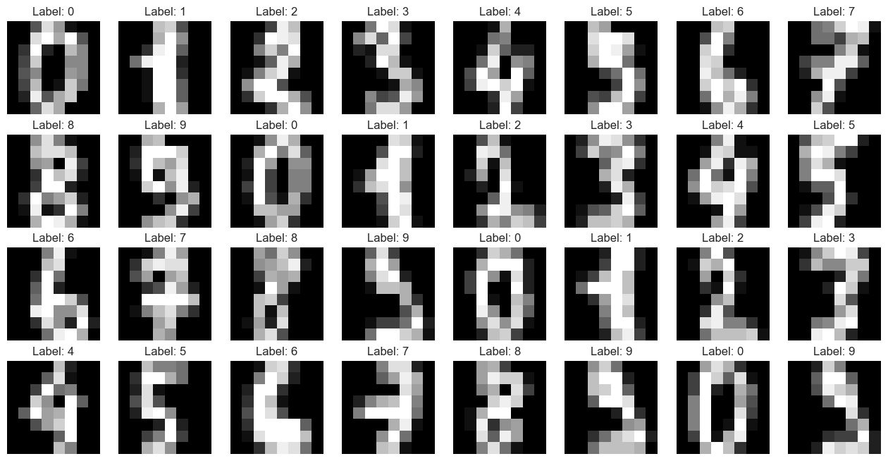
The visualisation of the digits data shows some samples of the handwritten digits:
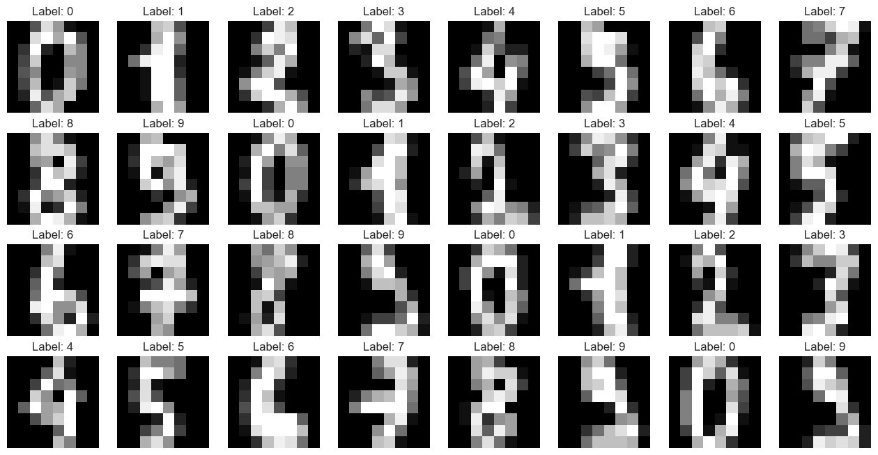
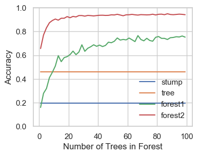
As a first introductory step, we estimate four basic tree models:
A stump model (i.e. a decision tree with max_depth=1)
A single tree model with max_depth=3
A forest model with 1 features and 1 depth level
A forest model with 2 features and max_depth=10
The accuracy of these models are plotted with the number of trees in the forest in the horizontal axis. The chart clearly shows that the more complex forrest model is superior in terms of accuracy.
from sklearn import ensemble

#%% Comparing Ensemble Methods
# Data:
digits = datasets.load_digits()
digits_ftrs, digits_tgt = digits.data, digits.target

# Visualising the Digits
fig, axes = plt.subplots(4, 8, figsize=(16, 8))
for i, ax in enumerate(axes.flat):
    ax.imshow(digits.images[i], cmap='gray')
    ax.set_title(f'Label: {digits.target[i]}')
    ax.axis('off')
plt.show()

def fit_predict_score(model, ds):
    return model_selection.cross_val_score(model, *ds, cv=10).mean()

stump = tree.DecisionTreeClassifier(max_depth=1)
dtree = tree.DecisionTreeClassifier(max_depth=3)
forest1 = ensemble.RandomForestClassifier(max_features=1, max_depth=1,n_jobs=-1)
forest2 = ensemble.RandomForestClassifier(max_features=2, max_depth=10,n_jobs=-1)

tree_classifiers = {'stump' : stump, 'dtree' : dtree, 'forest1': forest1, 'forest2': forest2}
max_est = 100

data = (digits_ftrs, digits_tgt)
stump_score = fit_predict_score(stump, data)
tree_score = fit_predict_score(dtree, data)

def interpolate_list(input_list, num_points):
    # Create an empty list to store the result
    interpolated_list = []

    # Loop through the list, interpolating between each pair of points
    for i in range(len(input_list) - 1):
        start = input_list[i]
        end = input_list[i + 1]
        # Interpolate between start and end
        interpolated_values = np.linspace(start, end, num_points, endpoint=False)
        # Add these interpolated values to the list, except the last one (to avoid duplication)
        interpolated_list.extend(interpolated_values)

    # Append the last element of the original list
    interpolated_list.append(input_list[-1])

    return interpolated_list

# This can be slow. We predict every other and then interpolate to speed it up.
forest1_scores = [fit_predict_score(forest1.set_params(n_estimators=n),
                                    data) for n in range(1,max_est+1,2)]
forest1_scores = interpolate_list(forest1_scores, 2)

# This can be slow. We predict every other and then interpolate to speed it up.
forest2_scores = [fit_predict_score(forest2.set_params(n_estimators=n),
                                    data) for n in range(1,max_est+1,2)]
forest2_scores = interpolate_list(forest2_scores, 2)
As in the case of the Iris model, we can visualise the decision tree as shown in the chart below for the decision tree model with max_depth=3.
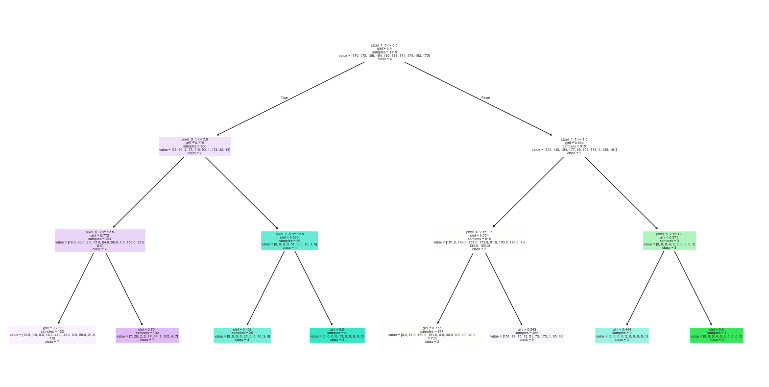
Furthermore, the confusion matrix is shown in the following heatmap chart (which clearly that our simple 3-level decision tree model had the most significant difficulties in identifying digit “8”)
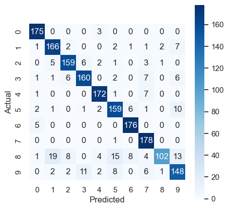
#We can view those results graphically:
fig, ax = plt.subplots(figsize=(4,3))
xs = list(range(1,max_est))
ax.plot(xs, np.repeat(stump_score, max_est-1), label='stump')
ax.plot(xs, np.repeat(tree_score, max_est-1), label='tree')
ax.plot(xs, forest1_scores, label='forest1')
ax.plot(xs, forest2_scores, label='forest2')
ax.set_xlabel('Number of Trees in Forest')
ax.set_ylabel('Accuracy')
ax.legend(loc='lower right');
ax.set_yticks([x * 0.2 for x in range(0, 6)])
#%% Can we also plot the decision tree for a single tree in Random Forest

# Fit the data to a particular tree
forest = ensemble.RandomForestClassifier(max_features=2, max_depth=3,
                                         n_jobs=-1, n_estimators = 50)
forest.fit(digits_ftrs,digits_tgt)
digits_pred = forest.fit(digits_ftrs,digits_tgt).predict(digits_ftrs)
plt.figure(figsize=(20,10))
tree.plot_tree(forest.estimators_[0], filled=True,
               feature_names=digits.feature_names,
               class_names=['0','1','2','3','4','5','6','7','8','9'])
plt.show()

# Compute a simple matrix that can be printed
cm = metrics.confusion_matrix(digits_tgt, digits_pred)
print("confusion matrix:", cm, sep="\n")

fig, ax = plt.subplots(1, 1, figsize=(5, 5))
ax = sns.heatmap(cm, annot=True, square=True,
                 xticklabels=['0','1','2','3','4','5','6','7','8','9'],
                 yticklabels=['0','1','2','3','4','5','6','7','8','9'],
                 fmt='d',
                 cmap='Blues')
ax.set_xlabel('Predicted')
ax.set_ylabel('Actual')
Features Importance#
Techniques that assign a score to each feature based on how useful they are at predicting the target variable. These scores indicate the relevance or impact of each feature in the model’s decision-making process.
Tree Based Models: Measure how much each feature contributes to reducing the impurity (like Gini impurity or entropy) in decision trees.
Permutation importance measures the increase in the model’s prediction error when the values of a particular feature are shuffled, breaking its relationship with the target. A larger increase in error indicates higher importance.
Model Improvement: Can focus on the most important features or by removing irrelevant ones which can reduce overfitting and improve generalization.
Bias and Caution: Can be biased if features are correlated or if the model is sensitive to certain types of features.
Which Features (Variables) Actually Matter? (Feature Importance)#
Understanding
forest.feature_importances_in Scikit-Learn
When moving from a single Decision Tree to a Random Forest (an ensemble of many trees), we lose the ability to easily draw and trace a single flowchart. However, we gain a powerful metric: Feature Importance.
In scikit-learn, calling .feature_importances_ on a trained Random Forest model returns an array of scores that quantify exactly how much each variable contributed to the model’s predictions.
Here is a breakdown of how it works and what it means for business strategy:
1. How It Is Calculated (Mean Decrease in Impurity)#
Every time a tree makes a split (like petal width <= 0.8), it reduces the “impurity” or chaos in the data (measured by the Gini score).
The algorithm tracks how much the Gini impurity decreased at that specific node.
It then multiplies that decrease by the proportion of data samples that passed through that node.
Finally, it sums up these weighted impurity decreases for each feature across all the trees in the forest and normalizes the final scores so they add up to 1.0 (or 100%).
2. The Business Intuition#
If the decision tree is the “how,” feature importance is the “what.” It directly answers the executive question: “Which KPIs are driving the outcomes?”
If TotalSpent has an importance score of 0.45 and Age has a score of 0.05, it means spending behavior is nine times more influential in predicting the outcome than the customer’s age. This allows managers to stop wasting resources tracking irrelevant metrics and focus their attention entirely on the high-impact variables.
3. A Critical Caveat for Analysts#
While highly useful, this specific scikit-learn metric (often called Gini Importance) has a known mathematical bias: it inflates the importance of continuous, high-cardinality features. If you have a feature with many unique values (like Income or an ID column), the trees have many more opportunities to split on it, which artificially inflates its final importance score. When dealing with mixed data types (e.g., combining continuous financial data with simple binary “Yes/No” flags), it is often better to use Permutation Importance to get a fairer assessment of what is actually driving the model.
For our “digits” example, the chart below show the importance of different features where each feature basically measures the light intensity of the respective pixel of the image representing the handwritten digit:
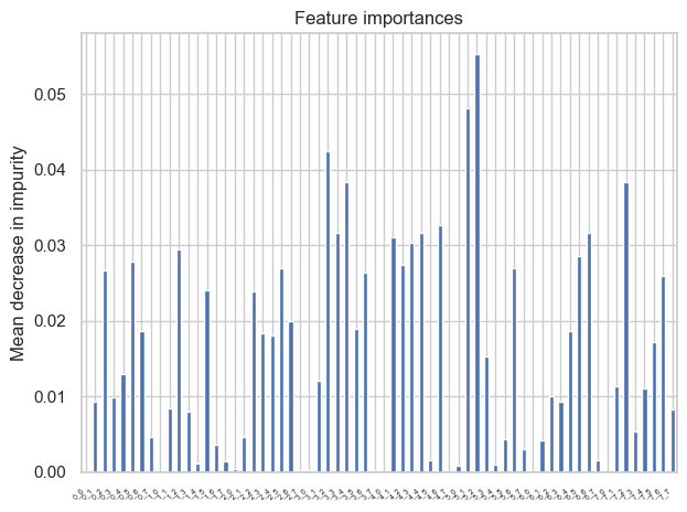
#%% Feature Importances
plt.figure(figsize=(20,10))

# Remove "pixel_" from the feature names to improve readability
feature_names = [s.replace("pixel_","") for s in digits.feature_names]
forest_importances = pd.Series(forest.feature_importances_, index=feature_names)

fig, ax = plt.subplots()
forest_importances.plot.bar(ax=ax)
ax.set_title("Feature importances")
ax.set_ylabel("Mean decrease in impurity")
ax.set_xticklabels(ax.get_xticklabels(), rotation=45, ha='right', fontsize=5)
fig.tight_layout()

plt.show()
LightGBM#
Boosting Concept: Decision trees are built sequentially. Each new tree tries to correct the errors made by previous.
Decision Trees (Grows Leaves): Grows trees leaf-wise, adds branches to leaves that contribute to reducing error.
Gradient Boosting: Each new tree is trained to reduce the residuals from the previous trees.
Histogram-Based Algorithm: Instead of evaluating all possible split points for each feature, it groups continuous values into discrete bins, reducing the number of splits to consider.
Efficient Handling of Large Datasets: It does this by leaf-wise tree growth and the histogram-based approach to reduce memory usage and computation time.
Handling Imbalanced Data: It can assign different weights to different classes, helping improve performance on tasks like fraud detection or rare event prediction.
Regularization: These techniques add penalties to the loss function to discourage the model from becoming too complex
Parallel and Distributed Training
Final Prediction: After all trees are built, the predictions from all the trees are combined by averaging or by voting
Why It Works: LightGBM is fast, efficient, and powerful. Its leaf-wise tree growth strategy allows it to capture complex patterns in the data, while its ability to handle large and imbalanced datasets makes it suitable for many real-world tasks.
XGBoost#
Boosting Concept: Decision trees are built sequentially. Each new tree is trained to correct the errors made by the previous trees.
Gradient Boosting: Each new tree is trained to reduce the residuals from the previous trees. This is done by optimizing a gradient loss function.
Additive Model: Trees are added one by one to the model. The prediction is made by summing up the outputs from all the trees.
Regularization: Regularization helps prevent overfitting by discouraging the model from becoming too complex.
Handling Missing Data: XGBoost can handle missing data internally. It automatically learns the best way to handle missing values during training.
Parallel Processing: XGBoost is designed to take advantage of modern computing capabilities, such as parallel processing.
Weighted Quantile Sketch: XGBoost uses a technique called weighted quantile sketch, which efficiently handles datasets with a large number of features or skewed data distributions.
Sparsity Awareness: XGBoost is optimized to handle sparse data. This makes it particularly useful for tasks like text classification or situations where features are encoded as one-hot vectors.
Final Prediction: Predictions from all the trees are summed up to give the final output. For classification tasks, the output is typically a probability, which can be converted into a class label. For regression tasks, it’s a continuous value.
Why It Works: XGBoost is powerful because it combines the strengths of gradient boosting with optimizations like regularization, parallel processing, and efficient handling of sparse and large datasets. These features make it accurate, fast, and scalable, which is why it’s widely used in machine learning competitions and real-world applications.
ExtraTrees#
Decision Trees: Based on decision trees.
Multiple Trees (Ensemble): Each tree is built using the entire dataset, but the splits in the trees are determined more randomly than in RF.
Random Splits: The algorithm picks a random subset of features and then selects a random split point for each feature. This randomness helps to reduce variance and overfitting.
No Bootstrap Sampling: Extra Trees does not use bootstrap sampling. Instead, each tree is trained on the entire dataset.
Fast and Efficient: Because Extra Trees doesn’t search for the optimal split at each node, it is generally faster to train than Random Forest.
Diversity Among Trees: The randomness in selecting split points across different features creates diverse trees within the ensemble.
Averaging (Regression) / Voting (Classification):
For classification tasks: The predictions from all the trees are combined by voting.
For regression tasks: The predictions from all the trees are averaged to produce the final prediction.
No Overfitting: Due to the high level of randomness, Extra Trees is less prone to overfitting.
Feature Importance: Extra Trees, like other tree-based methods, can be used to assess feature importance.
Why It Works: Extra Trees works well because it reduces variance through the use of random splits, which helps the model generalize better. It is particularly useful when you want a fast, efficient model that can handle large datasets with a low risk of overfitting.
Multi-Layer Perceptron Classifier (MLPC)#
Artificial Neural Network (ANN): It consists of layers of nodes (neurons) that are connected by weights.
Input Layer (first layer): Each neuron in this layer represents a feature from the dataset. The number of neurons in the input layer equals the input features.
Hidden Layers: Between the input and output layers are hidden layers. These layers process the inputs by applying a weighted sum of the inputs followed by an activation function (like ReLU, sigmoid, or tanh) to introduce non-linearity.
Output Layer (final layer): For classification tasks, the output layer typically has one neuron per class, and the output is a probability distribution over the classes, indicating the likelihood of each class.
Weights and Biases: Each connection between neurons has an associated weight, and each neuron has a bias term. These are adjusted during training to minimize the error in the model’s predictions.
Forward Propagation: During training, input data passes through the network from the input layer, through the hidden layers, and finally to the output layer. This process is called forward propagation, where each layer’s output becomes the input for the next layer.
Loss Function: The model uses a loss function (such as cross-entropy loss for classification tasks) to measure the difference between the predicted output and the actual target values. The goal is to minimize this loss during training.
Backpropagation: Backpropagation is the process used to train the network. It involves calculating the gradient of the loss function with respect to each weight and bias using the chain rule. These gradients are used to update the weights and biases to reduce the loss.
Activation Functions: Activation functions like ReLU (Rectified Linear Unit) or sigmoid are used in the hidden layers to introduce non-linearity, which enables the model to learn complex relationships in the data.
Final Prediction: After training, when a new data point is fed into the network, it goes through the same forward propagation process to produce a final prediction. For classification, this is typically the class with the highest probability in the output layer.
Why It Works: MLPC works well because it can model complex, non-linear relationships between features and the target variable. Its ability to learn from data through multiple layers allows it to perform well on a wide range of classification tasks.
More extensive ML models comparison for predicting digits#
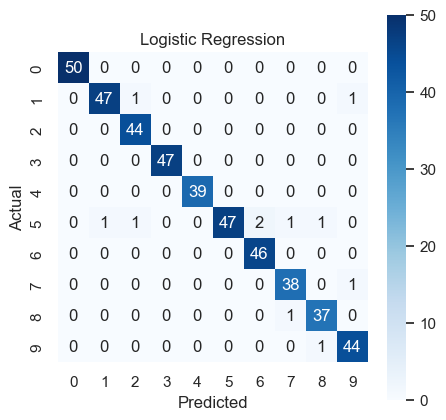
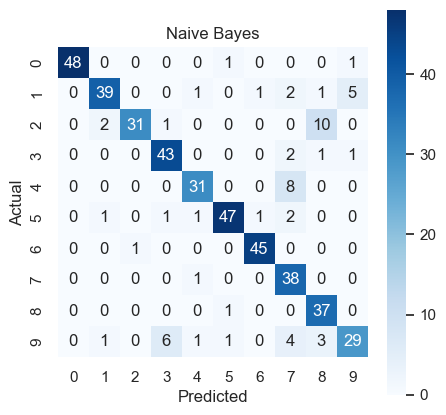
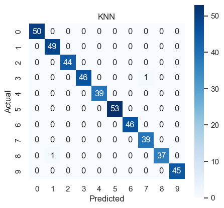
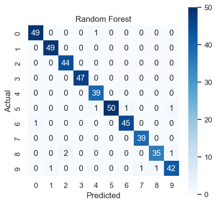
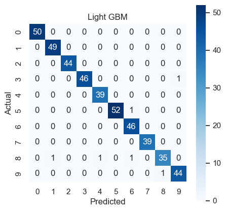
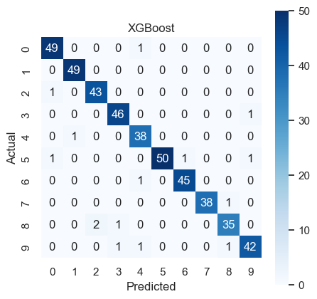
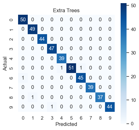
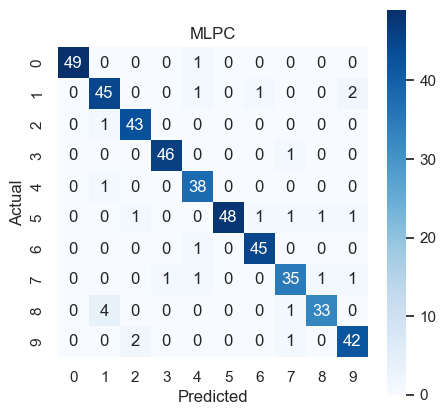
Now, let us consider a broader set of models from SKLEARN to predict digits and see how these models compare in terms of accuracy:
Logistic Regression
Naive Bayes Gaussian
KNN Classifier
Random Forest Classifier
LightGBM Classifier
XGBoost Classifier
ExtraTrees Classifier
Multi Layer Perceptron Classifier (MLPC)
To facilitate the comparisons, in the Python code below, we start by defining several wrapping functions, each of which basically calls the relevant sklearn function to produce, for example, confusion matrix and a set of other predictive performanc metrics. The same function will be called for each of the above ML models.
For each model, we supply default parameters value based on educated guess. Later we will implement hyperparameter tuning to see if we can squeeze out some noticeable improvements in the performance of the different models.
The results are summarised in the table below, which clearly shows that our lowly KNN performs the best, even when compared to the advanced ensemble models such as LightGBM and the neural network model such as MLPC.
Machine Learning Model Performance Comparison#
Model |
Accuracy |
Precision (Weighted) |
Recall (Weighted) |
F1-Score (Weighted) |
|---|---|---|---|---|
KNN |
99.56% |
99.57% |
99.56% |
99.56% |
Light GBM |
98.67% |
98.68% |
98.67% |
98.66% |
Extra Trees |
98.44% |
98.50% |
98.44% |
98.43% |
Random Forest |
97.56% |
97.63% |
97.56% |
97.54% |
Logistic Regression |
97.56% |
97.62% |
97.56% |
97.53% |
XGBoost |
96.67% |
96.71% |
96.67% |
96.66% |
MLPC |
94.44% |
94.63% |
94.44% |
94.40% |
Naive Bayes |
86.22% |
87.74% |
86.22% |
86.20% |
# More comparisons of various ML and Ensemble Models

# Some Custom Functions to simplify reuse with different model
def confusionMatrixDigits(y_test,y_pred,model):
    # Compute a simple matrix that can be printed
    cm = metrics.confusion_matrix(y_test, y_pred)
    print(f"Confusion Matrix ({model}):", cm, sep="\n")

    fig, ax = plt.subplots(1, 1, figsize=(5, 5))
    ax = sns.heatmap(cm, annot=True, square=True,
                     xticklabels=list(range(0,10)),
                     yticklabels=list(range(0,10)),
                     fmt='d',
                     cmap='Blues')
    ax.set_xlabel('Predicted')
    ax.set_ylabel('Actual')
    ax.set_title(model)

def metricSummary(predictTest,yTest,yPred,method):
    # Create a dictionary within the dictionary
    predictTest[method] = {}
    predictTest[method]['method'] = method
    predictTest[method]['accuracy'] = metrics.accuracy_score(yTest,yPred)
    temp = pd.DataFrame(metrics.precision_score(yTest,yPred,average=None)).T

    # We can calculate the precision for each digit
    for x in range(0,10):
        predictTest[method]['precision_' + str(x)] = temp[x][0]

    # Or we can average over all the possible classifications
    predictTest[method]['precision_Weighted'] = metrics.precision_score(yTest,yPred,average='weighted')

    temp = pd.DataFrame(metrics.recall_score(yTest,yPred,average=None)).T

    for x in range(0,10):
        predictTest[method]['recall_' + str(x)] = temp[x][0]
    predictTest[method]['recall_Weighted'] = metrics.recall_score(yTest,yPred,average='weighted')

    temp = pd.DataFrame(metrics.f1_score(yTest,yPred,average=None)).T
    for x in range(0,10):
        predictTest[method]['f1_' + str(x)] = temp[x][0]
    predictTest[method]['f1_Weighted'] = metrics.f1_score(yTest,yPred,average='weighted')

    return predictTest

def generalClassifier(classifier,parameters):
    # ** Unpacks the dictionary and passes each key value pair as a separate keyword
    return classifier(**parameters)

# Data:
digits = datasets.load_digits()

# Summarise the data
print(f"Mean Value: {np.mean(digits.data):.2f}")
print(f"Max Value: {np.max(digits.data):.2f}")
print(f"Min Value: {np.min(digits.data):.2f}")

# Visualising the Digits
fig, axes = plt.subplots(4, 8, figsize=(16, 8))
for i, ax in enumerate(axes.flat):
    ax.imshow(digits.images[i], cmap='gray')
    ax.set_title(f'Label: {digits.target[i]}')
    ax.axis('off')
plt.show()

# Split the data
(x_train, x_test, y_train, y_test) = train_test_split(digits.data,
                                                     digits.target,
                                                     test_size=0.25,
                                                     random_state=44)

# Create an empty dictionary to place assessment metrics
predictTest = {}
# A list of assessment metrics we will eventually store in a Pandas DF
columnList = ['method', 'accuracy']
# Assess the predictions for each classification
for var in ['precision_', 'recall_', 'f1_']:
    columnList += [var + str(x) for x in range(10)]
    columnList += [var + 'Weighted']

# A list of Estimators that we will compare
estimatorList = ['Logistic Regression', 'Naive Bayes',
                 'KNN', 'Random Forest',
                 'Light GBM', 'XGBoost',
                 'Extra Trees', 'MLPC']

# Let's set up some general parameters within a dictionary
# so we can cycle through to make our code a bit more efficient
paramDict = {}
for model in estimatorList:
    paramDict[model] = {}

paramDict['Logistic Regression']['params'] = {'max_iter': 1000,
                                              'solver': 'newton-cg'}
paramDict['Logistic Regression']['classifier'] = LogisticRegression

paramDict['Naive Bayes']['params'] = {}
paramDict['Naive Bayes']['classifier'] = naive_bayes.GaussianNB

paramDict['KNN']['params'] = {'n_neighbors': 10}
paramDict['KNN']['classifier'] = neighbors.KNeighborsClassifier

paramDict['Random Forest']['params'] = {'max_features': 2, 'max_depth': 10,
                                        'n_estimators': 100, 'n_jobs': -1}
paramDict['Random Forest']['classifier'] = ensemble.RandomForestClassifier

paramDict['Light GBM']['params'] = {'num_leaves': 31, 'n_estimators': 100,
                                    'objective': 'multiclass', 'verbose': -1}
paramDict['Light GBM']['classifier'] = lgb.LGBMClassifier

paramDict['XGBoost']['params'] = {'learning_rate': 0.5, 'max_depth': 10,
                                  'n_estimators': 100,
                                  'objective': 'multi:softmax', 'n_jobs': 1}
paramDict['XGBoost']['classifier'] = xgboost.XGBClassifier

paramDict['Extra Trees']['params'] = {'max_depth': 10, 'n_estimators': 100,
                                      'max_features': 0.5, 'n_jobs': 1}
paramDict['Extra Trees']['classifier'] = ensemble.ExtraTreesClassifier

paramDict['MLPC']['params'] = {'hidden_layer_sizes': (10,), 'max_iter': 2000,
                               'solver': 'adam', 'activation': 'logistic'}
paramDict['MLPC']['classifier'] = MLPClassifier

# With individual parameters set within the dictionary,
# let's loop over the models to make predictions and assess performance
for model in estimatorList:

    # Intialise the classifier
    classifier = generalClassifier(paramDict[model]['classifier'], paramDict[model]['params'])

    # Predict the values from the classifier
    y_pred = classifier.fit(x_train,y_train).predict(x_test)

    # Confusion Matrix
    confusionMatrixDigits(y_test,y_pred,model)

    # Output a series of metrics to assess the quality of the predictions
    predictTest = metricSummary(predictTest,y_test,y_pred,model)

# Convert the dictionary of metrics to a Pandas DataFrame
predictionTestOutput = pd.DataFrame.from_dict(predictTest, orient='index')

# Round the values to 3 digits and print out the index-value pairs
metricList = ['accuracy', 'precision_Weighted', 'recall_Weighted', 'f1_Weighted']
for metric in metricList:
    column = predictionTestOutput[metric]
    print(f"{metric}")
    for idx, value in column.items():
        print(f"{idx}: {value:.2%}")
    print()
Mean Value: 4.88
Max Value: 16.00
Min Value: 0.00
Confusion Matrix (Logistic Regression):
[[50  0  0  0  0  0  0  0  0  0]
 [ 0 47  1  0  0  0  0  0  0  1]
 [ 0  0 44  0  0  0  0  0  0  0]
 [ 0  0  0 47  0  0  0  0  0  0]
 [ 0  0  0  0 39  0  0  0  0  0]
 [ 0  1  1  0  0 47  2  1  1  0]
 [ 0  0  0  0  0  0 46  0  0  0]
 [ 0  0  0  0  0  0  0 38  0  1]
 [ 0  0  0  0  0  0  0  1 37  0]
 [ 0  0  0  0  0  0  0  0  1 44]]
Confusion Matrix (Naive Bayes):
[[48  0  0  0  0  1  0  0  0  1]
 [ 0 39  0  0  1  0  1  2  1  5]
 [ 0  2 31  1  0  0  0  0 10  0]
 [ 0  0  0 43  0  0  0  2  1  1]
 [ 0  0  0  0 31  0  0  8  0  0]
 [ 0  1  0  1  1 47  1  2  0  0]
 [ 0  0  1  0  0  0 45  0  0  0]
 [ 0  0  0  0  1  0  0 38  0  0]
 [ 0  0  0  0  0  1  0  0 37  0]
 [ 0  1  0  6  1  1  0  4  3 29]]
Confusion Matrix (KNN):
[[50  0  0  0  0  0  0  0  0  0]
 [ 0 49  0  0  0  0  0  0  0  0]
 [ 0  0 44  0  0  0  0  0  0  0]
 [ 0  0  0 46  0  0  0  1  0  0]
 [ 0  0  0  0 39  0  0  0  0  0]
 [ 0  0  0  0  0 53  0  0  0  0]
 [ 0  0  0  0  0  0 46  0  0  0]
 [ 0  0  0  0  0  0  0 39  0  0]
 [ 0  1  0  0  0  0  0  0 37  0]
 [ 0  0  0  0  0  0  0  0  0 45]]
Confusion Matrix (Random Forest):
[[49  0  0  0  1  0  0  0  0  0]
 [ 0 49  0  0  0  0  0  0  0  0]
 [ 0  0 44  0  0  0  0  0  0  0]
 [ 0  0  0 47  0  0  0  0  0  0]
 [ 0  0  0  0 39  0  0  0  0  0]
 [ 0  0  0  0  1 50  1  0  0  1]
 [ 1  0  0  0  0  0 45  0  0  0]
 [ 0  0  0  0  0  0  0 39  0  0]
 [ 0  0  2  0  0  0  0  0 35  1]
 [ 0  1  0  0  0  0  0  1  1 42]]
/opt/anaconda3/lib/python3.12/site-packages/sklearn/utils/validation.py:2749: UserWarning: X does not have valid feature names, but LGBMClassifier was fitted with feature names
  warnings.warn(
Confusion Matrix (Light GBM):
[[50  0  0  0  0  0  0  0  0  0]
 [ 0 49  0  0  0  0  0  0  0  0]
 [ 0  0 44  0  0  0  0  0  0  0]
 [ 0  0  0 46  0  0  0  0  0  1]
 [ 0  0  0  0 39  0  0  0  0  0]
 [ 0  0  0  0  0 52  1  0  0  0]
 [ 0  0  0  0  0  0 46  0  0  0]
 [ 0  0  0  0  0  0  0 39  0  0]
 [ 0  1  0  0  1  0  1  0 35  0]
 [ 0  0  0  0  0  0  0  0  1 44]]
Confusion Matrix (XGBoost):
[[49  0  0  0  1  0  0  0  0  0]
 [ 0 49  0  0  0  0  0  0  0  0]
 [ 1  0 43  0  0  0  0  0  0  0]
 [ 0  0  0 46  0  0  0  0  0  1]
 [ 0  1  0  0 38  0  0  0  0  0]
 [ 1  0  0  0  0 50  1  0  0  1]
 [ 0  0  0  0  1  0 45  0  0  0]
 [ 0  0  0  0  0  0  0 38  1  0]
 [ 0  0  2  1  0  0  0  0 35  0]
 [ 0  0  0  1  1  0  0  0  1 42]]
Confusion Matrix (Extra Trees):
[[50  0  0  0  0  0  0  0  0  0]
 [ 0 49  0  0  0  0  0  0  0  0]
 [ 0  0 44  0  0  0  0  0  0  0]
 [ 0  0  0 47  0  0  0  0  0  0]
 [ 0  0  0  0 39  0  0  0  0  0]
 [ 0  0  0  0  1 51  1  0  0  0]
 [ 1  0  0  0  0  0 45  0  0  0]
 [ 0  0  0  0  0  0  0 39  0  0]
 [ 0  1  0  0  0  0  0  0 37  0]
 [ 0  0  0  1  0  0  0  0  0 44]]
Confusion Matrix (MLPC):
[[49  0  0  0  1  0  0  0  0  0]
 [ 0 45  0  0  1  0  1  0  0  2]
 [ 0  1 43  0  0  0  0  0  0  0]
 [ 0  0  0 46  0  0  0  1  0  0]
 [ 0  1  0  0 38  0  0  0  0  0]
 [ 0  0  1  0  0 48  1  1  1  1]
 [ 0  0  0  0  1  0 45  0  0  0]
 [ 0  0  0  1  1  0  0 35  1  1]
 [ 0  4  0  0  0  0  0  1 33  0]
 [ 0  0  2  0  0  0  0  1  0 42]]
accuracy
Logistic Regression: 97.56%
Naive Bayes: 86.22%
KNN: 99.56%
Random Forest: 97.56%
Light GBM: 98.67%
XGBoost: 96.67%
Extra Trees: 98.89%
MLPC: 94.22%

precision_Weighted
Logistic Regression: 97.62%
Naive Bayes: 87.74%
KNN: 99.57%
Random Forest: 97.58%
Light GBM: 98.68%
XGBoost: 96.71%
Extra Trees: 98.91%
MLPC: 94.36%

recall_Weighted
Logistic Regression: 97.56%
Naive Bayes: 86.22%
KNN: 99.56%
Random Forest: 97.56%
Light GBM: 98.67%
XGBoost: 96.67%
Extra Trees: 98.89%
MLPC: 94.22%

f1_Weighted
Logistic Regression: 97.53%
Naive Bayes: 86.20%
KNN: 99.56%
Random Forest: 97.54%
Light GBM: 98.66%
XGBoost: 96.66%
Extra Trees: 98.89%
MLPC: 94.23%
Hyperparameter Tuning#
In the previous example, we set model parameters without any optimisation. In the last ML case study example shown below, we will attempt to tune the hyperparameters of each ML model using Bayesian optimization. This is called hyperparameter tuning.
There are several hyperparameter tuning functions provided by ML models, which include:
Grid Search: A methodical way of searching through a predefined set of hyperparameters.
Random Search: A more efficient method by randomly sampling the hyperparameter space.
Bayesian Optimization: Uses a probabilistic model to predict the performance of different hyperparameter sets.
Which hyperparameter tunining approach to choose depends on the trade-off between Time Complexity vs. Effectiveness.
Time Complexity: The amount of computational time required to complete the tuning process.
Influenced by the number of hyperparameters, size of search space, and model training time.
Effectiveness: How well the method finds the optimal or near-optimal set of hyperparameters. This is influenced by coverage of search space, and the balance between exploration and exploitation.
Essential Comparison of Methods:
Grid Search: High time complexity, effectiveness can vary based on the grid.
Random Search: Lower time complexity, often more effective in high-dimensional spaces.
Bayesian Optimization: Moderate time complexity, typically high effectiveness.
# Hyperparameter Tuning with Bayesian Search

import warnings
# Suppress the "The objective has been evaluated"". This is bad practice and should not be used in regular coding.
warnings.filterwarnings("ignore", category=UserWarning, message=".*The objective has been evaluated.*")


# Let's set up some general parameters within a dictionary so we can cycle through to make our code a bit more efficient
paramDict = {}
for model in estimatorList:
    paramDict[model] = {}

paramDict['Logistic Regression']['params'] = {'penalty': Categorical(['l2']),
                                              'C': Real(1e-6, 1e+6),
                                              'solver': Categorical(['newton-cg'])
                                              }

paramDict['Logistic Regression']['classifier'] = LogisticRegression

paramDict['Naive Bayes']['params'] = {'var_smoothing': Real(1e-09, 1e-02)}
paramDict['Naive Bayes']['classifier'] = naive_bayes.GaussianNB

paramDict['KNN']['params'] =  {'n_neighbors': Integer(1,100)}
paramDict['KNN']['classifier'] = neighbors.KNeighborsClassifier

paramDict['Random Forest']['params'] = {'n_estimators': Integer(10,1000),
                                        'min_samples_split': Integer(2,100),
                                        'min_samples_leaf': Integer(1,100),
                                        'max_features': Categorical(['sqrt','log2', 0.1, 0.2,
                                                                     0.3, 0.4, 0.5, 0.6, 0.7, 0.8, 0.9]),
                                        'max_leaf_nodes': Integer(2,100),
                                        'min_impurity_decrease': Real(0,2),
                                        'bootstrap': Categorical([True, False]),
                                        'ccp_alpha': Real(0,1e-2),
                                        'n_jobs': Categorical([1])
                                        }

paramDict['Random Forest']['classifier'] = ensemble.RandomForestClassifier

paramDict['Light GBM']['params'] = {'num_leaves': Integer(2,100),
                                    'n_jobs': Categorical([1]),
                                    'verbose': Categorical([-1]),
                                    'n_estimators': Integer(10,1000),
                                    'max_depth': Integer(1,26),
                                    'min_child_samples': Integer(15,100)
                                    }

paramDict['Light GBM']['classifier'] = lgb.LGBMClassifier

paramDict['XGBoost']['params'] = {'n_estimators': Integer(10,1000),
                                  'max_depth': Integer(1,26),
                                  'learning_rate': Real(1e-1,1),
                                  'objective': Categorical(['multi:softmax']),
                                  'n_jobs': Categorical([1]),
                                  'subsample': Real(1e-1,1),
                                  'gamma': Real(1e-1,3)
                                  }

paramDict['XGBoost']['classifier'] = xgboostclassifier = xgboost.XGBClassifier

paramDict['Extra Trees']['params'] = {'max_depth': Integer(1,52),
                                      'n_estimators': Integer(10,1000),
                                      'criterion': Categorical(['gini', 'entropy', 'log_loss']),
                                      'min_samples_split': Integer(2,100),
                                      'min_samples_leaf': Integer(1,100),
                                      'max_features': Categorical(['sqrt','log2', 0.1, 0.2, 0.3, 0.4, 0.5,
                                                                   0.6, 0.7, 0.8, 0.9])
                                      }

paramDict['Extra Trees']['classifier'] = xtrclassifier = ensemble.ExtraTreesClassifier

paramDict['MLPC']['params'] = {'alpha': Real(1e-2,1),
                               'max_iter': Integer(1000,10000),
                               'beta_1': Real(1e-2,0.9999),
                               'beta_2': Real(1e-2,0.9999)}

paramDict['MLPC']['classifier'] = mlpcclassifier = MLPClassifier

def customScorer(yTest,yPred):
    return metrics.f1_score(yTest,yPred,average='weighted')

nIter = 100 # This should be set higher in practice, we could get a really bad
            # distribution of parameters when this is set this low
scorerF1 = metrics.make_scorer(customScorer, greater_is_better=True)
# to save time we will use no cross validation: just one sample
# replace 1 with 5 if you want 5 fold cross validation with 2 (train and test) sample splits
# cv = RepeatedKFold(n_splits=5, n_repeats=5, random_state=0)
cv = RepeatedKFold(n_splits=2, n_repeats=1, random_state=0)
bestParameters = pd.DataFrame(index=np.arange(0), columns=['parameters','model'])

predictTestSearch = {}
# With individual parameters set within the dictionary,
# let's loop over the models to make predictions and assess performance

for model in estimatorList:
    print(f"Estimating Best Hyperparameter Model for the model: {model}")
    # Intialise the classifier
    cvModel = BayesSearchCV(generalClassifier(paramDict[model]['classifier'], {}),
                                     paramDict[model]['params'], random_state=0,
                                     n_iter=nIter, n_jobs=-1, scoring=scorerF1, cv=cv)

    # Predict the values from the classifier
    y_pred = cvModel.fit(x_train,y_train).predict(x_test)

    # Confusion Matrix
    modelUpdate = model + " CV Search"
    confusionMatrixDigits(y_test,y_pred,modelUpdate)

    # Output a series of metrics to assess the quality of the predictions
    predictTestSearch = metricSummary(predictTestSearch,y_test,y_pred,model)

    # Extract the parameters used
    temp = pd.DataFrame(index=np.arange(1), columns=['parameters','model'])
    temp['parameters'] = str(cvModel.best_params_)
    temp['model']= model
    bestParameters = pd.concat([bestParameters, temp], ignore_index=True)

    # Save the model for potential later deployment
    print(f"Best Hyperparameter Models for {model} is saved as: {model}.pkl")
    with open(model + ".pkl", "wb") as f:
        dump(cvModel.best_estimator_, f, protocol=5)

# Convert the dictionary of metrics to a Pandas DataFrame
predictionTestSearchOutput = pd.DataFrame.from_dict(predictTestSearch, orient='index')

# Round the values to 3 digits and print out the index-value pairs
metricList = ['accuracy', 'precision_Weighted', 'recall_Weighted', 'f1_Weighted']
for metric in metricList:
    column = predictionTestSearchOutput[metric].round(3)
    print(f"{metric}")
    for idx, value in column.items():
        print(f"{idx}: {value}")
    print()
Estimating Best Hyperparameter Model for the model: Logistic Regression
Confusion Matrix (Logistic Regression CV Search):
[[50  0  0  0  0  0  0  0  0  0]
 [ 0 46  1  0  1  0  0  0  0  1]
 [ 0  0 44  0  0  0  0  0  0  0]
 [ 0  0  1 46  0  0  0  0  0  0]
 [ 0  0  0  0 39  0  0  0  0  0]
 [ 0  1  1  0  0 47  2  1  1  0]
 [ 0  0  0  0  0  0 46  0  0  0]
 [ 0  0  0  0  1  0  0 37  0  1]
 [ 0  1  0  0  0  0  0  0 37  0]
 [ 0  0  0  0  0  0  1  0  1 43]]
Best Hyperparameter Models for Logistic Regression is saved as: Logistic Regression.pkl
Estimating Best Hyperparameter Model for the model: Naive Bayes
Confusion Matrix (Naive Bayes CV Search):
[[47  0  0  0  2  0  0  0  0  1]
 [ 0 36  2  0  1  0  0  1  3  6]
 [ 0  0 43  0  0  0  0  0  1  0]
 [ 0  0  0 43  0  0  0  1  2  1]
 [ 0  0  0  0 39  0  0  0  0  0]
 [ 0  1  0  1  1 48  1  0  0  1]
 [ 0  0  0  0  0  0 46  0  0  0]
 [ 0  0  0  0  0  0  0 38  1  0]
 [ 0  0  0  0  0  1  0  0 36  1]
 [ 0  1  0  1  1  0  0  3  1 38]]
Best Hyperparameter Models for Naive Bayes is saved as: Naive Bayes.pkl
Estimating Best Hyperparameter Model for the model: KNN
Confusion Matrix (KNN CV Search):
[[50  0  0  0  0  0  0  0  0  0]
 [ 0 49  0  0  0  0  0  0  0  0]
 [ 0  0 44  0  0  0  0  0  0  0]
 [ 0  0  0 47  0  0  0  0  0  0]
 [ 0  0  0  0 39  0  0  0  0  0]
 [ 0  0  0  0  0 51  1  0  0  1]
 [ 0  0  0  0  0  0 46  0  0  0]
 [ 0  0  0  0  0  0  0 39  0  0]
 [ 0  1  0  0  0  0  0  0 37  0]
 [ 0  0  0  0  0  0  0  0  1 44]]
Best Hyperparameter Models for KNN is saved as: KNN.pkl
Estimating Best Hyperparameter Model for the model: Random Forest
Confusion Matrix (Random Forest CV Search):
[[49  0  0  0  1  0  0  0  0  0]
 [ 0 49  0  0  0  0  0  0  0  0]
 [ 1  0 43  0  0  0  0  0  0  0]
 [ 0  0  0 47  0  0  0  0  0  0]
 [ 0  0  0  0 39  0  0  0  0  0]
 [ 0  0  0  0  1 50  1  0  0  1]
 [ 1  0  0  0  0  0 45  0  0  0]
 [ 0  0  0  0  0  0  0 38  1  0]
 [ 0  1  1  0  0  0  1  0 34  1]
 [ 0  0  0  0  0  0  0  0  1 44]]
Best Hyperparameter Models for Random Forest is saved as: Random Forest.pkl
Estimating Best Hyperparameter Model for the model: Light GBM
/opt/anaconda3/lib/python3.12/site-packages/sklearn/utils/validation.py:2749: UserWarning: X does not have valid feature names, but LGBMClassifier was fitted with feature names
  warnings.warn(
/opt/anaconda3/lib/python3.12/site-packages/sklearn/utils/validation.py:2749: UserWarning: X does not have valid feature names, but LGBMClassifier was fitted with feature names
  warnings.warn(
/opt/anaconda3/lib/python3.12/site-packages/sklearn/utils/validation.py:2749: UserWarning: X does not have valid feature names, but LGBMClassifier was fitted with feature names
  warnings.warn(
/opt/anaconda3/lib/python3.12/site-packages/sklearn/utils/validation.py:2749: UserWarning: X does not have valid feature names, but LGBMClassifier was fitted with feature names
  warnings.warn(
/opt/anaconda3/lib/python3.12/site-packages/sklearn/utils/validation.py:2749: UserWarning: X does not have valid feature names, but LGBMClassifier was fitted with feature names
  warnings.warn(
/opt/anaconda3/lib/python3.12/site-packages/sklearn/utils/validation.py:2749: UserWarning: X does not have valid feature names, but LGBMClassifier was fitted with feature names
  warnings.warn(
/opt/anaconda3/lib/python3.12/site-packages/sklearn/utils/validation.py:2749: UserWarning: X does not have valid feature names, but LGBMClassifier was fitted with feature names
  warnings.warn(
/opt/anaconda3/lib/python3.12/site-packages/sklearn/utils/validation.py:2749: UserWarning: X does not have valid feature names, but LGBMClassifier was fitted with feature names
  warnings.warn(
/opt/anaconda3/lib/python3.12/site-packages/sklearn/utils/validation.py:2749: UserWarning: X does not have valid feature names, but LGBMClassifier was fitted with feature names
  warnings.warn(
/opt/anaconda3/lib/python3.12/site-packages/sklearn/utils/validation.py:2749: UserWarning: X does not have valid feature names, but LGBMClassifier was fitted with feature names
  warnings.warn(
/opt/anaconda3/lib/python3.12/site-packages/sklearn/utils/validation.py:2749: UserWarning: X does not have valid feature names, but LGBMClassifier was fitted with feature names
  warnings.warn(
/opt/anaconda3/lib/python3.12/site-packages/sklearn/utils/validation.py:2749: UserWarning: X does not have valid feature names, but LGBMClassifier was fitted with feature names
  warnings.warn(
/opt/anaconda3/lib/python3.12/site-packages/sklearn/utils/validation.py:2749: UserWarning: X does not have valid feature names, but LGBMClassifier was fitted with feature names
  warnings.warn(
/opt/anaconda3/lib/python3.12/site-packages/sklearn/utils/validation.py:2749: UserWarning: X does not have valid feature names, but LGBMClassifier was fitted with feature names
  warnings.warn(
/opt/anaconda3/lib/python3.12/site-packages/sklearn/utils/validation.py:2749: UserWarning: X does not have valid feature names, but LGBMClassifier was fitted with feature names
  warnings.warn(
/opt/anaconda3/lib/python3.12/site-packages/sklearn/utils/validation.py:2749: UserWarning: X does not have valid feature names, but LGBMClassifier was fitted with feature names
  warnings.warn(
/opt/anaconda3/lib/python3.12/site-packages/sklearn/utils/validation.py:2749: UserWarning: X does not have valid feature names, but LGBMClassifier was fitted with feature names
  warnings.warn(
/opt/anaconda3/lib/python3.12/site-packages/sklearn/utils/validation.py:2749: UserWarning: X does not have valid feature names, but LGBMClassifier was fitted with feature names
  warnings.warn(
/opt/anaconda3/lib/python3.12/site-packages/sklearn/utils/validation.py:2749: UserWarning: X does not have valid feature names, but LGBMClassifier was fitted with feature names
  warnings.warn(
/opt/anaconda3/lib/python3.12/site-packages/sklearn/utils/validation.py:2749: UserWarning: X does not have valid feature names, but LGBMClassifier was fitted with feature names
  warnings.warn(
/opt/anaconda3/lib/python3.12/site-packages/sklearn/utils/validation.py:2749: UserWarning: X does not have valid feature names, but LGBMClassifier was fitted with feature names
  warnings.warn(
/opt/anaconda3/lib/python3.12/site-packages/sklearn/utils/validation.py:2749: UserWarning: X does not have valid feature names, but LGBMClassifier was fitted with feature names
  warnings.warn(
/opt/anaconda3/lib/python3.12/site-packages/sklearn/utils/validation.py:2749: UserWarning: X does not have valid feature names, but LGBMClassifier was fitted with feature names
  warnings.warn(
/opt/anaconda3/lib/python3.12/site-packages/sklearn/utils/validation.py:2749: UserWarning: X does not have valid feature names, but LGBMClassifier was fitted with feature names
  warnings.warn(
/opt/anaconda3/lib/python3.12/site-packages/sklearn/utils/validation.py:2749: UserWarning: X does not have valid feature names, but LGBMClassifier was fitted with feature names
  warnings.warn(
/opt/anaconda3/lib/python3.12/site-packages/sklearn/utils/validation.py:2749: UserWarning: X does not have valid feature names, but LGBMClassifier was fitted with feature names
  warnings.warn(
/opt/anaconda3/lib/python3.12/site-packages/sklearn/utils/validation.py:2749: UserWarning: X does not have valid feature names, but LGBMClassifier was fitted with feature names
  warnings.warn(
/opt/anaconda3/lib/python3.12/site-packages/sklearn/utils/validation.py:2749: UserWarning: X does not have valid feature names, but LGBMClassifier was fitted with feature names
  warnings.warn(
/opt/anaconda3/lib/python3.12/site-packages/sklearn/utils/validation.py:2749: UserWarning: X does not have valid feature names, but LGBMClassifier was fitted with feature names
  warnings.warn(
/opt/anaconda3/lib/python3.12/site-packages/sklearn/utils/validation.py:2749: UserWarning: X does not have valid feature names, but LGBMClassifier was fitted with feature names
  warnings.warn(
/opt/anaconda3/lib/python3.12/site-packages/sklearn/utils/validation.py:2749: UserWarning: X does not have valid feature names, but LGBMClassifier was fitted with feature names
  warnings.warn(
/opt/anaconda3/lib/python3.12/site-packages/sklearn/utils/validation.py:2749: UserWarning: X does not have valid feature names, but LGBMClassifier was fitted with feature names
  warnings.warn(
/opt/anaconda3/lib/python3.12/site-packages/sklearn/utils/validation.py:2749: UserWarning: X does not have valid feature names, but LGBMClassifier was fitted with feature names
  warnings.warn(
/opt/anaconda3/lib/python3.12/site-packages/sklearn/utils/validation.py:2749: UserWarning: X does not have valid feature names, but LGBMClassifier was fitted with feature names
  warnings.warn(
/opt/anaconda3/lib/python3.12/site-packages/sklearn/utils/validation.py:2749: UserWarning: X does not have valid feature names, but LGBMClassifier was fitted with feature names
  warnings.warn(
/opt/anaconda3/lib/python3.12/site-packages/sklearn/utils/validation.py:2749: UserWarning: X does not have valid feature names, but LGBMClassifier was fitted with feature names
  warnings.warn(
/opt/anaconda3/lib/python3.12/site-packages/sklearn/utils/validation.py:2749: UserWarning: X does not have valid feature names, but LGBMClassifier was fitted with feature names
  warnings.warn(
/opt/anaconda3/lib/python3.12/site-packages/sklearn/utils/validation.py:2749: UserWarning: X does not have valid feature names, but LGBMClassifier was fitted with feature names
  warnings.warn(
/opt/anaconda3/lib/python3.12/site-packages/sklearn/utils/validation.py:2749: UserWarning: X does not have valid feature names, but LGBMClassifier was fitted with feature names
  warnings.warn(
/opt/anaconda3/lib/python3.12/site-packages/sklearn/utils/validation.py:2749: UserWarning: X does not have valid feature names, but LGBMClassifier was fitted with feature names
  warnings.warn(
/opt/anaconda3/lib/python3.12/site-packages/sklearn/utils/validation.py:2749: UserWarning: X does not have valid feature names, but LGBMClassifier was fitted with feature names
  warnings.warn(
/opt/anaconda3/lib/python3.12/site-packages/sklearn/utils/validation.py:2749: UserWarning: X does not have valid feature names, but LGBMClassifier was fitted with feature names
  warnings.warn(
/opt/anaconda3/lib/python3.12/site-packages/sklearn/utils/validation.py:2749: UserWarning: X does not have valid feature names, but LGBMClassifier was fitted with feature names
  warnings.warn(
/opt/anaconda3/lib/python3.12/site-packages/sklearn/utils/validation.py:2749: UserWarning: X does not have valid feature names, but LGBMClassifier was fitted with feature names
  warnings.warn(
/opt/anaconda3/lib/python3.12/site-packages/sklearn/utils/validation.py:2749: UserWarning: X does not have valid feature names, but LGBMClassifier was fitted with feature names
  warnings.warn(
/opt/anaconda3/lib/python3.12/site-packages/sklearn/utils/validation.py:2749: UserWarning: X does not have valid feature names, but LGBMClassifier was fitted with feature names
  warnings.warn(
/opt/anaconda3/lib/python3.12/site-packages/sklearn/utils/validation.py:2749: UserWarning: X does not have valid feature names, but LGBMClassifier was fitted with feature names
  warnings.warn(
/opt/anaconda3/lib/python3.12/site-packages/sklearn/utils/validation.py:2749: UserWarning: X does not have valid feature names, but LGBMClassifier was fitted with feature names
  warnings.warn(
/opt/anaconda3/lib/python3.12/site-packages/sklearn/utils/validation.py:2749: UserWarning: X does not have valid feature names, but LGBMClassifier was fitted with feature names
  warnings.warn(
/opt/anaconda3/lib/python3.12/site-packages/sklearn/utils/validation.py:2749: UserWarning: X does not have valid feature names, but LGBMClassifier was fitted with feature names
  warnings.warn(
/opt/anaconda3/lib/python3.12/site-packages/sklearn/utils/validation.py:2749: UserWarning: X does not have valid feature names, but LGBMClassifier was fitted with feature names
  warnings.warn(
/opt/anaconda3/lib/python3.12/site-packages/sklearn/utils/validation.py:2749: UserWarning: X does not have valid feature names, but LGBMClassifier was fitted with feature names
  warnings.warn(
/opt/anaconda3/lib/python3.12/site-packages/sklearn/utils/validation.py:2749: UserWarning: X does not have valid feature names, but LGBMClassifier was fitted with feature names
  warnings.warn(
/opt/anaconda3/lib/python3.12/site-packages/sklearn/utils/validation.py:2749: UserWarning: X does not have valid feature names, but LGBMClassifier was fitted with feature names
  warnings.warn(
/opt/anaconda3/lib/python3.12/site-packages/sklearn/utils/validation.py:2749: UserWarning: X does not have valid feature names, but LGBMClassifier was fitted with feature names
  warnings.warn(
/opt/anaconda3/lib/python3.12/site-packages/sklearn/utils/validation.py:2749: UserWarning: X does not have valid feature names, but LGBMClassifier was fitted with feature names
  warnings.warn(
/opt/anaconda3/lib/python3.12/site-packages/sklearn/utils/validation.py:2749: UserWarning: X does not have valid feature names, but LGBMClassifier was fitted with feature names
  warnings.warn(
/opt/anaconda3/lib/python3.12/site-packages/sklearn/utils/validation.py:2749: UserWarning: X does not have valid feature names, but LGBMClassifier was fitted with feature names
  warnings.warn(
/opt/anaconda3/lib/python3.12/site-packages/sklearn/utils/validation.py:2749: UserWarning: X does not have valid feature names, but LGBMClassifier was fitted with feature names
  warnings.warn(
/opt/anaconda3/lib/python3.12/site-packages/sklearn/utils/validation.py:2749: UserWarning: X does not have valid feature names, but LGBMClassifier was fitted with feature names
  warnings.warn(
/opt/anaconda3/lib/python3.12/site-packages/sklearn/utils/validation.py:2749: UserWarning: X does not have valid feature names, but LGBMClassifier was fitted with feature names
  warnings.warn(
/opt/anaconda3/lib/python3.12/site-packages/sklearn/utils/validation.py:2749: UserWarning: X does not have valid feature names, but LGBMClassifier was fitted with feature names
  warnings.warn(
/opt/anaconda3/lib/python3.12/site-packages/sklearn/utils/validation.py:2749: UserWarning: X does not have valid feature names, but LGBMClassifier was fitted with feature names
  warnings.warn(
/opt/anaconda3/lib/python3.12/site-packages/sklearn/utils/validation.py:2749: UserWarning: X does not have valid feature names, but LGBMClassifier was fitted with feature names
  warnings.warn(
/opt/anaconda3/lib/python3.12/site-packages/sklearn/utils/validation.py:2749: UserWarning: X does not have valid feature names, but LGBMClassifier was fitted with feature names
  warnings.warn(
/opt/anaconda3/lib/python3.12/site-packages/sklearn/utils/validation.py:2749: UserWarning: X does not have valid feature names, but LGBMClassifier was fitted with feature names
  warnings.warn(
/opt/anaconda3/lib/python3.12/site-packages/sklearn/utils/validation.py:2749: UserWarning: X does not have valid feature names, but LGBMClassifier was fitted with feature names
  warnings.warn(
/opt/anaconda3/lib/python3.12/site-packages/sklearn/utils/validation.py:2749: UserWarning: X does not have valid feature names, but LGBMClassifier was fitted with feature names
  warnings.warn(
/opt/anaconda3/lib/python3.12/site-packages/sklearn/utils/validation.py:2749: UserWarning: X does not have valid feature names, but LGBMClassifier was fitted with feature names
  warnings.warn(
/opt/anaconda3/lib/python3.12/site-packages/sklearn/utils/validation.py:2749: UserWarning: X does not have valid feature names, but LGBMClassifier was fitted with feature names
  warnings.warn(
/opt/anaconda3/lib/python3.12/site-packages/sklearn/utils/validation.py:2749: UserWarning: X does not have valid feature names, but LGBMClassifier was fitted with feature names
  warnings.warn(
/opt/anaconda3/lib/python3.12/site-packages/sklearn/utils/validation.py:2749: UserWarning: X does not have valid feature names, but LGBMClassifier was fitted with feature names
  warnings.warn(
/opt/anaconda3/lib/python3.12/site-packages/sklearn/utils/validation.py:2749: UserWarning: X does not have valid feature names, but LGBMClassifier was fitted with feature names
  warnings.warn(
/opt/anaconda3/lib/python3.12/site-packages/sklearn/utils/validation.py:2749: UserWarning: X does not have valid feature names, but LGBMClassifier was fitted with feature names
  warnings.warn(
/opt/anaconda3/lib/python3.12/site-packages/sklearn/utils/validation.py:2749: UserWarning: X does not have valid feature names, but LGBMClassifier was fitted with feature names
  warnings.warn(
/opt/anaconda3/lib/python3.12/site-packages/sklearn/utils/validation.py:2749: UserWarning: X does not have valid feature names, but LGBMClassifier was fitted with feature names
  warnings.warn(
/opt/anaconda3/lib/python3.12/site-packages/sklearn/utils/validation.py:2749: UserWarning: X does not have valid feature names, but LGBMClassifier was fitted with feature names
  warnings.warn(
/opt/anaconda3/lib/python3.12/site-packages/sklearn/utils/validation.py:2749: UserWarning: X does not have valid feature names, but LGBMClassifier was fitted with feature names
  warnings.warn(
/opt/anaconda3/lib/python3.12/site-packages/sklearn/utils/validation.py:2749: UserWarning: X does not have valid feature names, but LGBMClassifier was fitted with feature names
  warnings.warn(
/opt/anaconda3/lib/python3.12/site-packages/sklearn/utils/validation.py:2749: UserWarning: X does not have valid feature names, but LGBMClassifier was fitted with feature names
  warnings.warn(
/opt/anaconda3/lib/python3.12/site-packages/sklearn/utils/validation.py:2749: UserWarning: X does not have valid feature names, but LGBMClassifier was fitted with feature names
  warnings.warn(
/opt/anaconda3/lib/python3.12/site-packages/sklearn/utils/validation.py:2749: UserWarning: X does not have valid feature names, but LGBMClassifier was fitted with feature names
  warnings.warn(
/opt/anaconda3/lib/python3.12/site-packages/sklearn/utils/validation.py:2749: UserWarning: X does not have valid feature names, but LGBMClassifier was fitted with feature names
  warnings.warn(
/opt/anaconda3/lib/python3.12/site-packages/sklearn/utils/validation.py:2749: UserWarning: X does not have valid feature names, but LGBMClassifier was fitted with feature names
  warnings.warn(
/opt/anaconda3/lib/python3.12/site-packages/sklearn/utils/validation.py:2749: UserWarning: X does not have valid feature names, but LGBMClassifier was fitted with feature names
  warnings.warn(
/opt/anaconda3/lib/python3.12/site-packages/sklearn/utils/validation.py:2749: UserWarning: X does not have valid feature names, but LGBMClassifier was fitted with feature names
  warnings.warn(
/opt/anaconda3/lib/python3.12/site-packages/sklearn/utils/validation.py:2749: UserWarning: X does not have valid feature names, but LGBMClassifier was fitted with feature names
  warnings.warn(
/opt/anaconda3/lib/python3.12/site-packages/sklearn/utils/validation.py:2749: UserWarning: X does not have valid feature names, but LGBMClassifier was fitted with feature names
  warnings.warn(
/opt/anaconda3/lib/python3.12/site-packages/sklearn/utils/validation.py:2749: UserWarning: X does not have valid feature names, but LGBMClassifier was fitted with feature names
  warnings.warn(
/opt/anaconda3/lib/python3.12/site-packages/sklearn/utils/validation.py:2749: UserWarning: X does not have valid feature names, but LGBMClassifier was fitted with feature names
  warnings.warn(
/opt/anaconda3/lib/python3.12/site-packages/sklearn/utils/validation.py:2749: UserWarning: X does not have valid feature names, but LGBMClassifier was fitted with feature names
  warnings.warn(
/opt/anaconda3/lib/python3.12/site-packages/sklearn/utils/validation.py:2749: UserWarning: X does not have valid feature names, but LGBMClassifier was fitted with feature names
  warnings.warn(
/opt/anaconda3/lib/python3.12/site-packages/sklearn/utils/validation.py:2749: UserWarning: X does not have valid feature names, but LGBMClassifier was fitted with feature names
  warnings.warn(
/opt/anaconda3/lib/python3.12/site-packages/sklearn/utils/validation.py:2749: UserWarning: X does not have valid feature names, but LGBMClassifier was fitted with feature names
  warnings.warn(
/opt/anaconda3/lib/python3.12/site-packages/sklearn/utils/validation.py:2749: UserWarning: X does not have valid feature names, but LGBMClassifier was fitted with feature names
  warnings.warn(
/opt/anaconda3/lib/python3.12/site-packages/sklearn/utils/validation.py:2749: UserWarning: X does not have valid feature names, but LGBMClassifier was fitted with feature names
  warnings.warn(
/opt/anaconda3/lib/python3.12/site-packages/sklearn/utils/validation.py:2749: UserWarning: X does not have valid feature names, but LGBMClassifier was fitted with feature names
  warnings.warn(
/opt/anaconda3/lib/python3.12/site-packages/sklearn/utils/validation.py:2749: UserWarning: X does not have valid feature names, but LGBMClassifier was fitted with feature names
  warnings.warn(
/opt/anaconda3/lib/python3.12/site-packages/sklearn/utils/validation.py:2749: UserWarning: X does not have valid feature names, but LGBMClassifier was fitted with feature names
  warnings.warn(
/opt/anaconda3/lib/python3.12/site-packages/sklearn/utils/validation.py:2749: UserWarning: X does not have valid feature names, but LGBMClassifier was fitted with feature names
  warnings.warn(
/opt/anaconda3/lib/python3.12/site-packages/sklearn/utils/validation.py:2749: UserWarning: X does not have valid feature names, but LGBMClassifier was fitted with feature names
  warnings.warn(
/opt/anaconda3/lib/python3.12/site-packages/sklearn/utils/validation.py:2749: UserWarning: X does not have valid feature names, but LGBMClassifier was fitted with feature names
  warnings.warn(
/opt/anaconda3/lib/python3.12/site-packages/sklearn/utils/validation.py:2749: UserWarning: X does not have valid feature names, but LGBMClassifier was fitted with feature names
  warnings.warn(
/opt/anaconda3/lib/python3.12/site-packages/sklearn/utils/validation.py:2749: UserWarning: X does not have valid feature names, but LGBMClassifier was fitted with feature names
  warnings.warn(
/opt/anaconda3/lib/python3.12/site-packages/sklearn/utils/validation.py:2749: UserWarning: X does not have valid feature names, but LGBMClassifier was fitted with feature names
  warnings.warn(
/opt/anaconda3/lib/python3.12/site-packages/sklearn/utils/validation.py:2749: UserWarning: X does not have valid feature names, but LGBMClassifier was fitted with feature names
  warnings.warn(
/opt/anaconda3/lib/python3.12/site-packages/sklearn/utils/validation.py:2749: UserWarning: X does not have valid feature names, but LGBMClassifier was fitted with feature names
  warnings.warn(
/opt/anaconda3/lib/python3.12/site-packages/sklearn/utils/validation.py:2749: UserWarning: X does not have valid feature names, but LGBMClassifier was fitted with feature names
  warnings.warn(
/opt/anaconda3/lib/python3.12/site-packages/sklearn/utils/validation.py:2749: UserWarning: X does not have valid feature names, but LGBMClassifier was fitted with feature names
  warnings.warn(
/opt/anaconda3/lib/python3.12/site-packages/sklearn/utils/validation.py:2749: UserWarning: X does not have valid feature names, but LGBMClassifier was fitted with feature names
  warnings.warn(
/opt/anaconda3/lib/python3.12/site-packages/sklearn/utils/validation.py:2749: UserWarning: X does not have valid feature names, but LGBMClassifier was fitted with feature names
  warnings.warn(
/opt/anaconda3/lib/python3.12/site-packages/sklearn/utils/validation.py:2749: UserWarning: X does not have valid feature names, but LGBMClassifier was fitted with feature names
  warnings.warn(
/opt/anaconda3/lib/python3.12/site-packages/sklearn/utils/validation.py:2749: UserWarning: X does not have valid feature names, but LGBMClassifier was fitted with feature names
  warnings.warn(
/opt/anaconda3/lib/python3.12/site-packages/sklearn/utils/validation.py:2749: UserWarning: X does not have valid feature names, but LGBMClassifier was fitted with feature names
  warnings.warn(
/opt/anaconda3/lib/python3.12/site-packages/sklearn/utils/validation.py:2749: UserWarning: X does not have valid feature names, but LGBMClassifier was fitted with feature names
  warnings.warn(
/opt/anaconda3/lib/python3.12/site-packages/sklearn/utils/validation.py:2749: UserWarning: X does not have valid feature names, but LGBMClassifier was fitted with feature names
  warnings.warn(
/opt/anaconda3/lib/python3.12/site-packages/sklearn/utils/validation.py:2749: UserWarning: X does not have valid feature names, but LGBMClassifier was fitted with feature names
  warnings.warn(
/opt/anaconda3/lib/python3.12/site-packages/sklearn/utils/validation.py:2749: UserWarning: X does not have valid feature names, but LGBMClassifier was fitted with feature names
  warnings.warn(
/opt/anaconda3/lib/python3.12/site-packages/sklearn/utils/validation.py:2749: UserWarning: X does not have valid feature names, but LGBMClassifier was fitted with feature names
  warnings.warn(
/opt/anaconda3/lib/python3.12/site-packages/sklearn/utils/validation.py:2749: UserWarning: X does not have valid feature names, but LGBMClassifier was fitted with feature names
  warnings.warn(
/opt/anaconda3/lib/python3.12/site-packages/sklearn/utils/validation.py:2749: UserWarning: X does not have valid feature names, but LGBMClassifier was fitted with feature names
  warnings.warn(
/opt/anaconda3/lib/python3.12/site-packages/sklearn/utils/validation.py:2749: UserWarning: X does not have valid feature names, but LGBMClassifier was fitted with feature names
  warnings.warn(
/opt/anaconda3/lib/python3.12/site-packages/sklearn/utils/validation.py:2749: UserWarning: X does not have valid feature names, but LGBMClassifier was fitted with feature names
  warnings.warn(
/opt/anaconda3/lib/python3.12/site-packages/sklearn/utils/validation.py:2749: UserWarning: X does not have valid feature names, but LGBMClassifier was fitted with feature names
  warnings.warn(
/opt/anaconda3/lib/python3.12/site-packages/sklearn/utils/validation.py:2749: UserWarning: X does not have valid feature names, but LGBMClassifier was fitted with feature names
  warnings.warn(
/opt/anaconda3/lib/python3.12/site-packages/sklearn/utils/validation.py:2749: UserWarning: X does not have valid feature names, but LGBMClassifier was fitted with feature names
  warnings.warn(
/opt/anaconda3/lib/python3.12/site-packages/sklearn/utils/validation.py:2749: UserWarning: X does not have valid feature names, but LGBMClassifier was fitted with feature names
  warnings.warn(
/opt/anaconda3/lib/python3.12/site-packages/sklearn/utils/validation.py:2749: UserWarning: X does not have valid feature names, but LGBMClassifier was fitted with feature names
  warnings.warn(
/opt/anaconda3/lib/python3.12/site-packages/sklearn/utils/validation.py:2749: UserWarning: X does not have valid feature names, but LGBMClassifier was fitted with feature names
  warnings.warn(
/opt/anaconda3/lib/python3.12/site-packages/sklearn/utils/validation.py:2749: UserWarning: X does not have valid feature names, but LGBMClassifier was fitted with feature names
  warnings.warn(
/opt/anaconda3/lib/python3.12/site-packages/sklearn/utils/validation.py:2749: UserWarning: X does not have valid feature names, but LGBMClassifier was fitted with feature names
  warnings.warn(
/opt/anaconda3/lib/python3.12/site-packages/sklearn/utils/validation.py:2749: UserWarning: X does not have valid feature names, but LGBMClassifier was fitted with feature names
  warnings.warn(
/opt/anaconda3/lib/python3.12/site-packages/sklearn/utils/validation.py:2749: UserWarning: X does not have valid feature names, but LGBMClassifier was fitted with feature names
  warnings.warn(
/opt/anaconda3/lib/python3.12/site-packages/sklearn/utils/validation.py:2749: UserWarning: X does not have valid feature names, but LGBMClassifier was fitted with feature names
  warnings.warn(
/opt/anaconda3/lib/python3.12/site-packages/sklearn/utils/validation.py:2749: UserWarning: X does not have valid feature names, but LGBMClassifier was fitted with feature names
  warnings.warn(
/opt/anaconda3/lib/python3.12/site-packages/sklearn/utils/validation.py:2749: UserWarning: X does not have valid feature names, but LGBMClassifier was fitted with feature names
  warnings.warn(
/opt/anaconda3/lib/python3.12/site-packages/sklearn/utils/validation.py:2749: UserWarning: X does not have valid feature names, but LGBMClassifier was fitted with feature names
  warnings.warn(
/opt/anaconda3/lib/python3.12/site-packages/sklearn/utils/validation.py:2749: UserWarning: X does not have valid feature names, but LGBMClassifier was fitted with feature names
  warnings.warn(
/opt/anaconda3/lib/python3.12/site-packages/sklearn/utils/validation.py:2749: UserWarning: X does not have valid feature names, but LGBMClassifier was fitted with feature names
  warnings.warn(
/opt/anaconda3/lib/python3.12/site-packages/sklearn/utils/validation.py:2749: UserWarning: X does not have valid feature names, but LGBMClassifier was fitted with feature names
  warnings.warn(
/opt/anaconda3/lib/python3.12/site-packages/sklearn/utils/validation.py:2749: UserWarning: X does not have valid feature names, but LGBMClassifier was fitted with feature names
  warnings.warn(
/opt/anaconda3/lib/python3.12/site-packages/sklearn/utils/validation.py:2749: UserWarning: X does not have valid feature names, but LGBMClassifier was fitted with feature names
  warnings.warn(
/opt/anaconda3/lib/python3.12/site-packages/sklearn/utils/validation.py:2749: UserWarning: X does not have valid feature names, but LGBMClassifier was fitted with feature names
  warnings.warn(
/opt/anaconda3/lib/python3.12/site-packages/sklearn/utils/validation.py:2749: UserWarning: X does not have valid feature names, but LGBMClassifier was fitted with feature names
  warnings.warn(
/opt/anaconda3/lib/python3.12/site-packages/sklearn/utils/validation.py:2749: UserWarning: X does not have valid feature names, but LGBMClassifier was fitted with feature names
  warnings.warn(
/opt/anaconda3/lib/python3.12/site-packages/sklearn/utils/validation.py:2749: UserWarning: X does not have valid feature names, but LGBMClassifier was fitted with feature names
  warnings.warn(
/opt/anaconda3/lib/python3.12/site-packages/sklearn/utils/validation.py:2749: UserWarning: X does not have valid feature names, but LGBMClassifier was fitted with feature names
  warnings.warn(
/opt/anaconda3/lib/python3.12/site-packages/sklearn/utils/validation.py:2749: UserWarning: X does not have valid feature names, but LGBMClassifier was fitted with feature names
  warnings.warn(
/opt/anaconda3/lib/python3.12/site-packages/sklearn/utils/validation.py:2749: UserWarning: X does not have valid feature names, but LGBMClassifier was fitted with feature names
  warnings.warn(
/opt/anaconda3/lib/python3.12/site-packages/sklearn/utils/validation.py:2749: UserWarning: X does not have valid feature names, but LGBMClassifier was fitted with feature names
  warnings.warn(
/opt/anaconda3/lib/python3.12/site-packages/sklearn/utils/validation.py:2749: UserWarning: X does not have valid feature names, but LGBMClassifier was fitted with feature names
  warnings.warn(
/opt/anaconda3/lib/python3.12/site-packages/sklearn/utils/validation.py:2749: UserWarning: X does not have valid feature names, but LGBMClassifier was fitted with feature names
  warnings.warn(
/opt/anaconda3/lib/python3.12/site-packages/sklearn/utils/validation.py:2749: UserWarning: X does not have valid feature names, but LGBMClassifier was fitted with feature names
  warnings.warn(
/opt/anaconda3/lib/python3.12/site-packages/sklearn/utils/validation.py:2749: UserWarning: X does not have valid feature names, but LGBMClassifier was fitted with feature names
  warnings.warn(
/opt/anaconda3/lib/python3.12/site-packages/sklearn/utils/validation.py:2749: UserWarning: X does not have valid feature names, but LGBMClassifier was fitted with feature names
  warnings.warn(
/opt/anaconda3/lib/python3.12/site-packages/sklearn/utils/validation.py:2749: UserWarning: X does not have valid feature names, but LGBMClassifier was fitted with feature names
  warnings.warn(
/opt/anaconda3/lib/python3.12/site-packages/sklearn/utils/validation.py:2749: UserWarning: X does not have valid feature names, but LGBMClassifier was fitted with feature names
  warnings.warn(
/opt/anaconda3/lib/python3.12/site-packages/sklearn/utils/validation.py:2749: UserWarning: X does not have valid feature names, but LGBMClassifier was fitted with feature names
  warnings.warn(
/opt/anaconda3/lib/python3.12/site-packages/sklearn/utils/validation.py:2749: UserWarning: X does not have valid feature names, but LGBMClassifier was fitted with feature names
  warnings.warn(
/opt/anaconda3/lib/python3.12/site-packages/sklearn/utils/validation.py:2749: UserWarning: X does not have valid feature names, but LGBMClassifier was fitted with feature names
  warnings.warn(
/opt/anaconda3/lib/python3.12/site-packages/sklearn/utils/validation.py:2749: UserWarning: X does not have valid feature names, but LGBMClassifier was fitted with feature names
  warnings.warn(
/opt/anaconda3/lib/python3.12/site-packages/sklearn/utils/validation.py:2749: UserWarning: X does not have valid feature names, but LGBMClassifier was fitted with feature names
  warnings.warn(
/opt/anaconda3/lib/python3.12/site-packages/sklearn/utils/validation.py:2749: UserWarning: X does not have valid feature names, but LGBMClassifier was fitted with feature names
  warnings.warn(
/opt/anaconda3/lib/python3.12/site-packages/sklearn/utils/validation.py:2749: UserWarning: X does not have valid feature names, but LGBMClassifier was fitted with feature names
  warnings.warn(
/opt/anaconda3/lib/python3.12/site-packages/sklearn/utils/validation.py:2749: UserWarning: X does not have valid feature names, but LGBMClassifier was fitted with feature names
  warnings.warn(
/opt/anaconda3/lib/python3.12/site-packages/sklearn/utils/validation.py:2749: UserWarning: X does not have valid feature names, but LGBMClassifier was fitted with feature names
  warnings.warn(
/opt/anaconda3/lib/python3.12/site-packages/sklearn/utils/validation.py:2749: UserWarning: X does not have valid feature names, but LGBMClassifier was fitted with feature names
  warnings.warn(
/opt/anaconda3/lib/python3.12/site-packages/sklearn/utils/validation.py:2749: UserWarning: X does not have valid feature names, but LGBMClassifier was fitted with feature names
  warnings.warn(
/opt/anaconda3/lib/python3.12/site-packages/sklearn/utils/validation.py:2749: UserWarning: X does not have valid feature names, but LGBMClassifier was fitted with feature names
  warnings.warn(
/opt/anaconda3/lib/python3.12/site-packages/sklearn/utils/validation.py:2749: UserWarning: X does not have valid feature names, but LGBMClassifier was fitted with feature names
  warnings.warn(
/opt/anaconda3/lib/python3.12/site-packages/sklearn/utils/validation.py:2749: UserWarning: X does not have valid feature names, but LGBMClassifier was fitted with feature names
  warnings.warn(
/opt/anaconda3/lib/python3.12/site-packages/sklearn/utils/validation.py:2749: UserWarning: X does not have valid feature names, but LGBMClassifier was fitted with feature names
  warnings.warn(
/opt/anaconda3/lib/python3.12/site-packages/sklearn/utils/validation.py:2749: UserWarning: X does not have valid feature names, but LGBMClassifier was fitted with feature names
  warnings.warn(
/opt/anaconda3/lib/python3.12/site-packages/sklearn/utils/validation.py:2749: UserWarning: X does not have valid feature names, but LGBMClassifier was fitted with feature names
  warnings.warn(
/opt/anaconda3/lib/python3.12/site-packages/sklearn/utils/validation.py:2749: UserWarning: X does not have valid feature names, but LGBMClassifier was fitted with feature names
  warnings.warn(
/opt/anaconda3/lib/python3.12/site-packages/sklearn/utils/validation.py:2749: UserWarning: X does not have valid feature names, but LGBMClassifier was fitted with feature names
  warnings.warn(
/opt/anaconda3/lib/python3.12/site-packages/sklearn/utils/validation.py:2749: UserWarning: X does not have valid feature names, but LGBMClassifier was fitted with feature names
  warnings.warn(
/opt/anaconda3/lib/python3.12/site-packages/sklearn/utils/validation.py:2749: UserWarning: X does not have valid feature names, but LGBMClassifier was fitted with feature names
  warnings.warn(
/opt/anaconda3/lib/python3.12/site-packages/sklearn/utils/validation.py:2749: UserWarning: X does not have valid feature names, but LGBMClassifier was fitted with feature names
  warnings.warn(
/opt/anaconda3/lib/python3.12/site-packages/sklearn/utils/validation.py:2749: UserWarning: X does not have valid feature names, but LGBMClassifier was fitted with feature names
  warnings.warn(
/opt/anaconda3/lib/python3.12/site-packages/sklearn/utils/validation.py:2749: UserWarning: X does not have valid feature names, but LGBMClassifier was fitted with feature names
  warnings.warn(
/opt/anaconda3/lib/python3.12/site-packages/sklearn/utils/validation.py:2749: UserWarning: X does not have valid feature names, but LGBMClassifier was fitted with feature names
  warnings.warn(
/opt/anaconda3/lib/python3.12/site-packages/sklearn/utils/validation.py:2749: UserWarning: X does not have valid feature names, but LGBMClassifier was fitted with feature names
  warnings.warn(
/opt/anaconda3/lib/python3.12/site-packages/sklearn/utils/validation.py:2749: UserWarning: X does not have valid feature names, but LGBMClassifier was fitted with feature names
  warnings.warn(
/opt/anaconda3/lib/python3.12/site-packages/sklearn/utils/validation.py:2749: UserWarning: X does not have valid feature names, but LGBMClassifier was fitted with feature names
  warnings.warn(
/opt/anaconda3/lib/python3.12/site-packages/sklearn/utils/validation.py:2749: UserWarning: X does not have valid feature names, but LGBMClassifier was fitted with feature names
  warnings.warn(
/opt/anaconda3/lib/python3.12/site-packages/sklearn/utils/validation.py:2749: UserWarning: X does not have valid feature names, but LGBMClassifier was fitted with feature names
  warnings.warn(
/opt/anaconda3/lib/python3.12/site-packages/sklearn/utils/validation.py:2749: UserWarning: X does not have valid feature names, but LGBMClassifier was fitted with feature names
  warnings.warn(
/opt/anaconda3/lib/python3.12/site-packages/sklearn/utils/validation.py:2749: UserWarning: X does not have valid feature names, but LGBMClassifier was fitted with feature names
  warnings.warn(
/opt/anaconda3/lib/python3.12/site-packages/sklearn/utils/validation.py:2749: UserWarning: X does not have valid feature names, but LGBMClassifier was fitted with feature names
  warnings.warn(
/opt/anaconda3/lib/python3.12/site-packages/sklearn/utils/validation.py:2749: UserWarning: X does not have valid feature names, but LGBMClassifier was fitted with feature names
  warnings.warn(
/opt/anaconda3/lib/python3.12/site-packages/sklearn/utils/validation.py:2749: UserWarning: X does not have valid feature names, but LGBMClassifier was fitted with feature names
  warnings.warn(
/opt/anaconda3/lib/python3.12/site-packages/sklearn/utils/validation.py:2749: UserWarning: X does not have valid feature names, but LGBMClassifier was fitted with feature names
  warnings.warn(
/opt/anaconda3/lib/python3.12/site-packages/sklearn/utils/validation.py:2749: UserWarning: X does not have valid feature names, but LGBMClassifier was fitted with feature names
  warnings.warn(
/opt/anaconda3/lib/python3.12/site-packages/sklearn/utils/validation.py:2749: UserWarning: X does not have valid feature names, but LGBMClassifier was fitted with feature names
  warnings.warn(
/opt/anaconda3/lib/python3.12/site-packages/sklearn/utils/validation.py:2749: UserWarning: X does not have valid feature names, but LGBMClassifier was fitted with feature names
  warnings.warn(
/opt/anaconda3/lib/python3.12/site-packages/sklearn/utils/validation.py:2749: UserWarning: X does not have valid feature names, but LGBMClassifier was fitted with feature names
  warnings.warn(
/opt/anaconda3/lib/python3.12/site-packages/sklearn/utils/validation.py:2749: UserWarning: X does not have valid feature names, but LGBMClassifier was fitted with feature names
  warnings.warn(
/opt/anaconda3/lib/python3.12/site-packages/sklearn/utils/validation.py:2749: UserWarning: X does not have valid feature names, but LGBMClassifier was fitted with feature names
  warnings.warn(
/opt/anaconda3/lib/python3.12/site-packages/sklearn/utils/validation.py:2749: UserWarning: X does not have valid feature names, but LGBMClassifier was fitted with feature names
  warnings.warn(
/opt/anaconda3/lib/python3.12/site-packages/sklearn/utils/validation.py:2749: UserWarning: X does not have valid feature names, but LGBMClassifier was fitted with feature names
  warnings.warn(
Confusion Matrix (Light GBM CV Search):
[[50  0  0  0  0  0  0  0  0  0]
 [ 0 48  0  0  0  0  0  0  0  1]
 [ 0  0 44  0  0  0  0  0  0  0]
 [ 0  0  0 46  0  0  0  0  0  1]
 [ 0  0  0  0 39  0  0  0  0  0]
 [ 0  0  0  0  0 50  2  0  0  1]
 [ 0  0  0  0  0  0 46  0  0  0]
 [ 0  0  0  0  0  0  0 38  1  0]
 [ 0  1  1  0  0  0  0  0 35  1]
 [ 0  0  0  0  0  0  0  0  1 44]]
Best Hyperparameter Models for Light GBM is saved as: Light GBM.pkl
Estimating Best Hyperparameter Model for the model: XGBoost
/opt/anaconda3/lib/python3.12/site-packages/joblib/externals/loky/process_executor.py:752: UserWarning: A worker stopped while some jobs were given to the executor. This can be caused by a too short worker timeout or by a memory leak.
  warnings.warn(
Confusion Matrix (XGBoost CV Search):
[[50  0  0  0  0  0  0  0  0  0]
 [ 0 49  0  0  0  0  0  0  0  0]
 [ 0  0 44  0  0  0  0  0  0  0]
 [ 0  0  0 47  0  0  0  0  0  0]
 [ 0  0  0  0 39  0  0  0  0  0]
 [ 0  0  0  0  0 52  1  0  0  0]
 [ 1  0  0  0  0  0 45  0  0  0]
 [ 0  0  0  0  0  0  0 38  1  0]
 [ 0  1  1  0  0  0  0  0 35  1]
 [ 0  0  0  0  0  0  0  0  0 45]]
Best Hyperparameter Models for XGBoost is saved as: XGBoost.pkl
Estimating Best Hyperparameter Model for the model: Extra Trees
Confusion Matrix (Extra Trees CV Search):
[[50  0  0  0  0  0  0  0  0  0]
 [ 0 49  0  0  0  0  0  0  0  0]
 [ 0  0 44  0  0  0  0  0  0  0]
 [ 0  0  0 47  0  0  0  0  0  0]
 [ 0  0  0  0 39  0  0  0  0  0]
 [ 0  0  0  0  1 51  1  0  0  0]
 [ 0  0  0  0  0  0 46  0  0  0]
 [ 0  0  0  0  0  0  0 39  0  0]
 [ 0  1  1  0  0  0  0  0 36  0]
 [ 0  0  0  0  0  0  0  0  0 45]]
Best Hyperparameter Models for Extra Trees is saved as: Extra Trees.pkl
Estimating Best Hyperparameter Model for the model: MLPC
Confusion Matrix (MLPC CV Search):
[[50  0  0  0  0  0  0  0  0  0]
 [ 0 49  0  0  0  0  0  0  0  0]
 [ 0  0 44  0  0  0  0  0  0  0]
 [ 0  0  0 47  0  0  0  0  0  0]
 [ 0  0  0  0 39  0  0  0  0  0]
 [ 0  1  1  0  1 49  1  0  0  0]
 [ 0  0  0  0  0  0 46  0  0  0]
 [ 0  0  0  0  0  0  0 38  1  0]
 [ 0  1  0  0  0  0  0  0 37  0]
 [ 0  0  0  0  0  0  0  0  0 45]]
Best Hyperparameter Models for MLPC is saved as: MLPC.pkl
accuracy
Logistic Regression: 0.967
Naive Bayes: 0.92
KNN: 0.991
Random Forest: 0.973
Light GBM: 0.978
XGBoost: 0.987
Extra Trees: 0.991
MLPC: 0.987

precision_Weighted
Logistic Regression: 0.968
Naive Bayes: 0.925
KNN: 0.991
Random Forest: 0.974
Light GBM: 0.978
XGBoost: 0.987
Extra Trees: 0.991
MLPC: 0.987

recall_Weighted
Logistic Regression: 0.967
Naive Bayes: 0.92
KNN: 0.991
Random Forest: 0.973
Light GBM: 0.978
XGBoost: 0.987
Extra Trees: 0.991
MLPC: 0.987

f1_Weighted
Logistic Regression: 0.966
Naive Bayes: 0.92
KNN: 0.991
Random Forest: 0.973
Light GBM: 0.978
XGBoost: 0.987
Extra Trees: 0.991
MLPC: 0.987
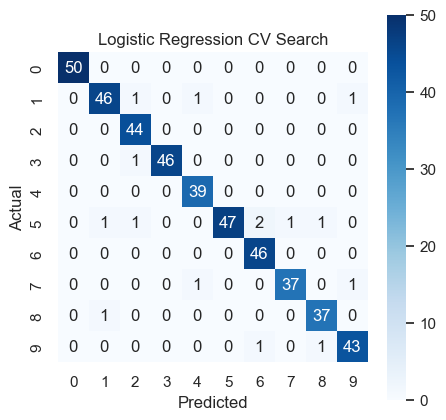
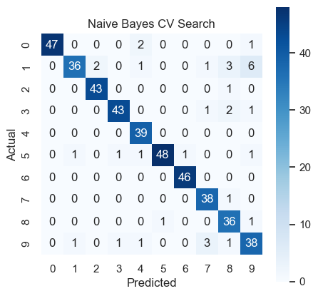
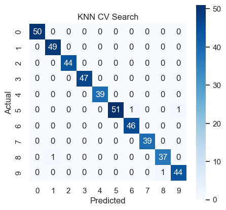
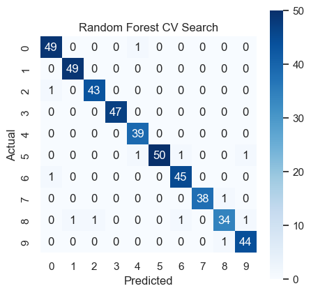
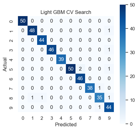
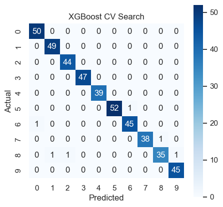
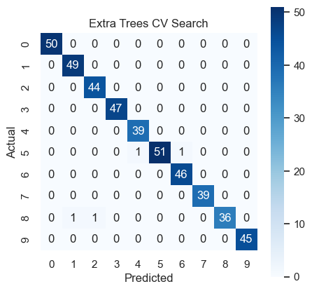
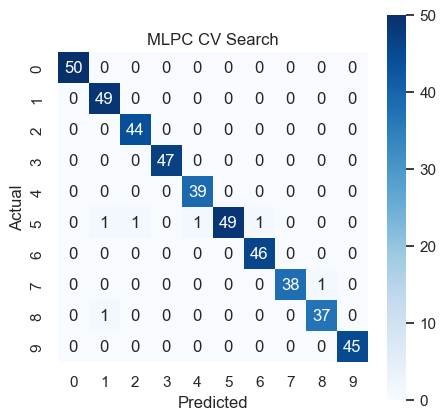
Deployment of Machine Learning Models#
Once we are happy with a specific machine learning model, we can save the model into a Pickle file and deploy it to be use to produce predictions based on new features data.
In the previous hyperparameter tuning codes, we have saved the hypertuned models using the following parts of the codes:
    # Save the model for potential later deployment
    print(f"Best Hyperparameter Models for {model} is saved as: {model}.pkl")
    with open(model + ".pkl", "wb") as f:
        dump(cvModel.best_estimator_, f, protocol=5)
The output of the above codes includes, for example, “KNN.pkl”, “Logistic Regression.pkl”, and “XGBoost.pkl”.
In the following example, we deploy each of these models to a new set of handwritten digits images prepared by Trevor.
# First, we load Trevor's handwriting data, which is in the same format as the digits data we have been using.
# We will use the models we have just saved to predict the digits in Trevor's handwriting and assess the
# performance of those predictions.

# Creating a subfolder in the current directory to hold Trevor's handwritten digit images
current_directory = os.getcwd()
image_output_directory = 'trevor_images'
# Create a folder in the current directory
os.makedirs(image_output_directory, exist_ok=True)

# Trevor's handwrittend images are in zippef file which we need to unzip
with zipfile.ZipFile('trevor-digits.zip', 'r') as zips:
    zips.extractall(image_output_directory)

# Concatenate the set of digits I created from the zipfile
images = []
for file in os.listdir(image_output_directory):
    if file.endswith('.png'):
        images.append(os.path.join(image_output_directory,file))

# Load images
images = [mpimg.imread(img_path) for img_path in images]

# Cycle through the images and add to a subplot
fig, axs = plt.subplots(7, 10, figsize=(20, 14))
for i, ax in enumerate(axs.ravel()):
    ax.imshow(images[i])
    ax.axis('off')  # Turn off axis labels

plt.show()

# We need to do a bit of clean up on these images to try and ensure they
# are as close as possible to the original

# Open an image and take the red channel into a one dimensional array
def redChannel(image_path):
    image = Image.open(image_path)
    image_array = np.array(image)
    return image_array[:,:,0].flatten()

trevorWriting = pd.DataFrame()

# As the label is in the file name, we will loop over and obtain all of the
for x in range(0,10):
    matching_files = []

    # Find all images with the value in its filename
    for file in os.listdir(image_output_directory):
        if str(x) in file and file.endswith('.png'):
            matching_files.append(file)

    for file in matching_files:
        image = redChannel(os.path.join(image_output_directory,file))
        temp = pd.Series(image, name=str(x))
        trevorWriting = pd.concat([trevorWriting,temp], axis=1)

# Transpose the data to be conformable with the existing digits data
trevorData = trevorWriting.T.reset_index() # This creates a column called index that has the target value
trevorTarget = pd.DataFrame()
trevorTarget['target'] = trevorData['index'].astype(int)
trevorData.drop('index', axis=1, inplace=True)

print(f"Max Value of features before rescaling: {trevorData.max().max()}")

# We want to normalise each image so there is some maximum value that
# equals 16 to correspond to the max value for each digit in the original
def normalise_row(row):
    max_value = row.max() # Find the maximum value in the row
    return row / max_value # Divide all values in the row by the max

# Normalising the row
trevorData = trevorData.apply(normalise_row, axis=1)
trevorData = (trevorData * 16).astype(int)

print(f"Max Value of features after rescaling: {trevorData.max().max()}")


# Deploying Saved Models and using them to predict my handwriting

for model in estimatorList:

    with open(model + '.pkl', 'rb') as f:
        modelLoad = load(f)

    y_pred = modelLoad.fit(x_train,y_train).predict(trevorData)

    confusionMatrixDigits(trevorTarget,y_pred,model + " (External Digits)")

    print(f"{model} accuracy: {metrics.accuracy_score(trevorTarget, y_pred):.2%}")
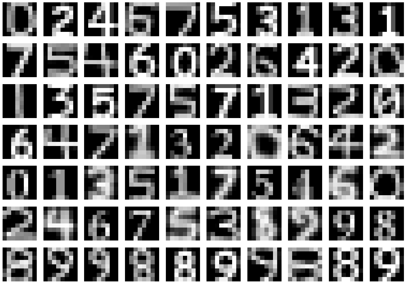
Max Value of features before rescaling: 255
Max Value of features after rescaling: 16
Confusion Matrix (Logistic Regression (External Digits)):
[[2 0 2 2 0 0 1 0 0 0]
 [0 3 3 1 0 0 0 0 0 0]
 [0 0 7 0 0 0 0 0 0 0]
 [0 0 0 7 0 0 0 0 0 0]
 [0 1 0 1 5 0 0 0 0 0]
 [0 0 0 1 0 6 0 0 0 0]
 [0 0 0 2 0 2 3 0 0 0]
 [0 0 1 0 0 0 0 6 0 0]
 [0 0 0 1 2 0 0 0 4 0]
 [1 0 0 0 3 0 0 0 0 3]]
Logistic Regression accuracy: 65.71%
Confusion Matrix (Naive Bayes (External Digits)):
[[4 0 2 0 0 0 0 0 0 1]
 [0 3 4 0 0 0 0 0 0 0]
 [0 0 6 0 0 0 0 0 0 1]
 [0 0 3 2 0 0 0 0 0 2]
 [0 1 0 0 4 1 0 0 1 0]
 [0 0 0 0 0 5 0 0 1 1]
 [0 0 0 0 2 3 2 0 0 0]
 [0 0 0 0 0 0 0 7 0 0]
 [0 0 1 2 0 1 0 0 3 0]
 [0 0 0 0 1 0 0 1 0 5]]
Naive Bayes accuracy: 58.57%
Confusion Matrix (KNN (External Digits)):
[[7 0 0 0 0 0 0 0 0 0]
 [0 3 4 0 0 0 0 0 0 0]
 [0 0 7 0 0 0 0 0 0 0]
 [0 0 0 6 0 0 0 0 0 1]
 [0 2 0 0 5 0 0 0 0 0]
 [0 0 0 0 0 5 0 0 0 2]
 [0 0 0 0 0 4 3 0 0 0]
 [0 0 0 0 0 0 0 7 0 0]
 [0 0 0 0 0 1 0 0 3 3]
 [1 0 0 0 0 2 0 0 0 4]]
KNN accuracy: 71.43%
Confusion Matrix (Random Forest (External Digits)):
[[5 0 0 0 0 0 0 0 1 1]
 [0 3 4 0 0 0 0 0 0 0]
 [0 0 7 0 0 0 0 0 0 0]
 [0 0 0 5 0 1 0 0 0 1]
 [0 1 0 0 4 0 0 1 0 1]
 [0 0 0 0 0 5 0 0 0 2]
 [1 0 0 1 1 2 2 0 0 0]
 [0 0 0 1 0 0 0 6 0 0]
 [1 0 0 0 0 0 1 0 4 1]
 [0 0 0 0 1 2 0 0 1 3]]
Random Forest accuracy: 62.86%
Confusion Matrix (Light GBM (External Digits)):
[[4 0 1 1 0 0 0 0 1 0]
 [0 3 3 1 0 0 0 0 0 0]
 [0 0 7 0 0 0 0 0 0 0]
 [0 0 0 5 0 1 0 1 0 0]
 [0 1 0 2 4 0 0 0 0 0]
 [0 0 0 0 1 6 0 0 0 0]
 [0 0 0 2 1 3 1 0 0 0]
 [0 0 0 1 0 0 0 6 0 0]
 [0 0 0 0 0 1 0 0 4 2]
 [0 0 0 0 2 2 0 0 0 3]]
Light GBM accuracy: 61.43%
Confusion Matrix (XGBoost (External Digits)):
[[4 0 0 2 0 1 0 0 0 0]
 [0 3 3 1 0 0 0 0 0 0]
 [0 0 7 0 0 0 0 0 0 0]
 [0 0 0 5 0 1 0 1 0 0]
 [0 1 0 2 4 0 0 0 0 0]
 [0 0 0 0 0 6 0 0 0 1]
 [0 0 0 2 1 2 2 0 0 0]
 [0 0 0 0 0 1 0 6 0 0]
 [0 0 0 0 0 2 0 0 4 1]
 [0 0 0 0 2 4 0 0 0 1]]
XGBoost accuracy: 60.00%
Confusion Matrix (Extra Trees (External Digits)):
[[7 0 0 0 0 0 0 0 0 0]
 [0 3 4 0 0 0 0 0 0 0]
 [0 0 7 0 0 0 0 0 0 0]
 [0 0 0 6 0 0 0 0 0 1]
 [0 3 0 0 4 0 0 0 0 0]
 [0 0 0 0 0 6 0 0 0 1]
 [0 0 0 1 1 3 2 0 0 0]
 [0 0 0 0 0 0 0 7 0 0]
 [0 0 0 0 0 0 1 0 4 2]
 [1 0 0 0 1 2 0 0 0 3]]
Extra Trees accuracy: 70.00%
Confusion Matrix (MLPC (External Digits)):
[[4 0 2 1 0 0 0 0 0 0]
 [0 3 3 1 0 0 0 0 0 0]
 [0 0 7 0 0 0 0 0 0 0]
 [0 0 0 6 0 0 0 1 0 0]
 [0 1 0 2 4 0 0 0 0 0]
 [0 0 0 1 0 5 0 0 0 1]
 [0 0 0 2 1 2 2 0 0 0]
 [0 0 1 1 0 0 0 5 0 0]
 [0 0 0 0 0 0 0 1 4 2]
 [0 0 0 0 2 0 0 2 0 3]]
MLPC accuracy: 61.43%
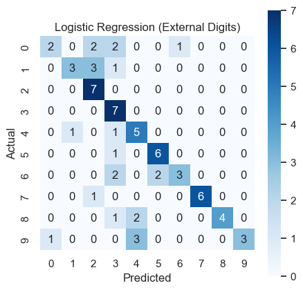
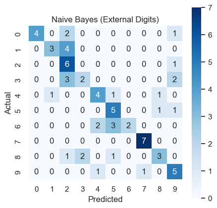
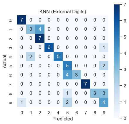
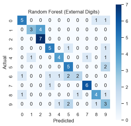
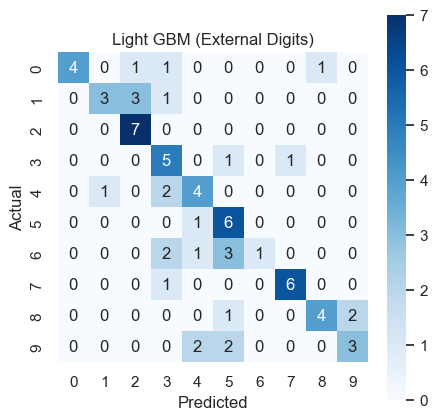
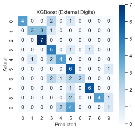
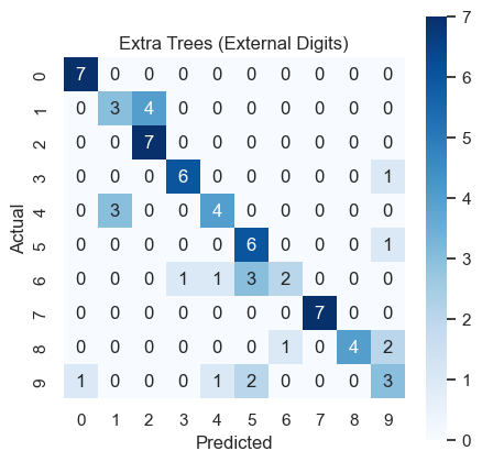
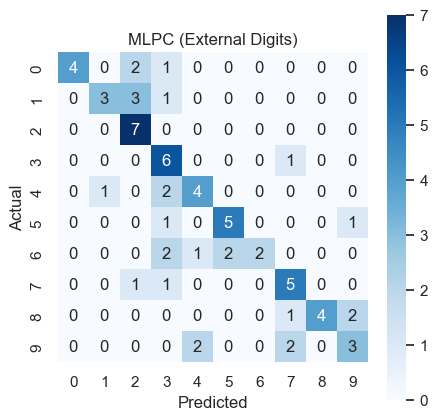
Unsupervised Learning#
Machine learning model that learns patterns from data without label (i.e. no predefined answers or categories)
Supervised learning: train a model using input-output pairs
Unsupervised learning: the algorithm explore the data on its own to discover hidden structures or relationships.
Common Types of Unsupervised Learning:#
Clustering
Goal: Group similar data points together (e.g. customer segmentation based on purchasing behavior)
Algorithms: K-Means, Hierarchical Clustering, DBSCAN
Dimensionality Reduction
Goal: Reduce the number of features (variables) while preserving important information (e.g. for simplifying data or removing noise)
Algorithms: Principal Component Analysis (PCA), t-SNE (t-distributed Stochastic Neighbour Embedding), Autoencoders (a type of Neural Network)
Association Rule Learning
Goal: Discover relationships between different variables (e.g., targeted discounts: customers who bought diapers often also bought baby food; product placement at supermarket)
Algorithm: Apriori (if an itemset is frequent, then all of its subset is frequent), FP-Growth (Frequent Pattern Tree)
Anomaly Detection
Goal: Identify rare or unusual data points that differ significantly from the majority
Application Examples for Unsupervised Learning Models#
Banking: Fraud detection (Anomaly detection with “Isolation Forest” model)
Healthcare: Patient subtyping e.g. diabetes types (Clustering with K-means on lab results)
Entertainment: Movie/music recommendation based on discovered user taste groups (Clustering + dimensionality reduction)
Manufacturing: Detecting defective products from sensor data (Autoencoders: reconstruction error = anomaly))
Case Project: Customer Segmentation Using Clustering#
1. Why is Customer Segmentation Important?#
In data-driven business environment, companies can improve their business performance by using data to derive a better understanding of their custormers. Different customers have different characteristics, behaviors, and preferences, which result in differences in their overall business value to the companies. Ignoring such heterogeneity in customers by, for example, relying only on a single overall average measure of the customer such as based on mean income or total sales can masks the true potentials for an optimal business value creation. As a result, suboptimal and generic marketing strategies where, for example, the same marekting promotions are offered to all custormers regardless of their chraracteristics.
With relatively easy to collect cutormer characteristics data, data-driven methods, such as clustering, are available to be implemented to identify hidden patterns and group customers with similar behaviors without relying on the existence of a label or predefined categories. The resulting insights from such unsupervised learning model can lead to better targeted strategies to increase business performance and improve the customer experience.
In this Case Prokect, we will use the data to ilustrate the implementation of unsupervised learning method:
Principal Component Analysis (PCA)
K-Means Clustering Analysis,
DBSCAN Clustering Analysis, and
Hieararchical Clustering
In Step 1 below, we will start with importing the relevant modules
# Intialise the modules we will use
import pandas as pd
import numpy as np
import matplotlib.pyplot as plt
import seaborn as sns
from sklearn.preprocessing import StandardScaler
from sklearn.decomposition import PCA
from sklearn.cluster import KMeans, DBSCAN
from sklearn.neighbors import NearestNeighbors

# Set plotting style for professional business reports
plt.style.use('seaborn-v0_8-whitegrid')
2: Dataset & Data Preparation#
Dataset Overview
The dataset originates from a Kaggle Customer Segmentation project. Original Structure: 2,240 rows and 29 columns. Features: Includes demographics (Birth Year, Education, Marital Status, Income, Children) and behavioral metrics (Recency, spending across categories like Wines, Fruits, Meat, and Gold). Engagement Metrics: Tracks web visits, catalog purchases, store purchases, and responses to multiple marketing campaigns.
For this example, we will use the “marketing_campagn.csv” data downloaded from Kaggle (https://www.kaggle.com/datasets/vishakhdapat/customer-segmentation-clustering). As described in the linked Kaggle page, the marketing campaign data file contains a rich set of information for conducting Customer Personality Analysis. The complete list of features in the CSV formattted data file includes, for examples:
Id: Unique identifier for each individual in the dataset.
Year_Birth: The birth year of the individual.
Education: The highest level of education attained by the individual.
Income: The annual income of the individual.
Dt_Customer: The date when the customer was first enrolled or became a part of the company’s database.
Recency: The number of days since the last purchase or interaction.
NumDealsPurchases: The number of purchases made with a discount or as part of a deal.
NumWebPurchases: The number of purchases made through the company’s website.
AcceptedCmp3: Binary indicator (1 or 0) whether the individual accepted the third marketing campaign.
Complain: Binary indicator (1 or 0) whether the individual has made a complaint.
Z_CostContact: A constant cost associated with contacting a customer.
Z_Revenue: A constant revenue associated with a successful campaign response.
Response: Binary indicator (1 or 0) whether the individual responded to the marketing campaign.
Step 2 performs Data Loading & Initial Cleaning and Feature Engineering
Feature Engineering: We combine several numerical features to create aggregated metrics, such as calculating the total amount spent across all product categories and summing the total campaign interactions. After cleaning the data and engineering these features, the final dataset consists of 2,216 rows and 20 columns.
# Load the dataset (Assuming 'customer_segmentation.csv' is in your working directory)
df = pd.read_csv('2024HB5notes/customer_segmentation.csv')
print(df.columns)

# 1. Clean Data: Drop rows with missing 'Income' values
df = df.dropna(subset=['Income'])

# 2. Feature Engineering
# Calculate Age
df['Age'] = 2024 - df['Year_Birth']

# Calculate Total Spending
df['TotalSpent'] = df[['MntWines', 'MntFruits', 'MntMeatProducts', 'MntFishProducts', 'MntSweetProducts', 'MntGoldProds']].sum(axis=1)

# Calculate Total Campaign Acceptance
df['TotalAccCmp'] = df[['AcceptedCmp1', 'AcceptedCmp2', 'AcceptedCmp3', 'AcceptedCmp4', 'AcceptedCmp5', 'Response']].sum(axis=1)

print(f"Cleaned dataset shape: {df.shape}")
3: Data Exploration Insights#
Exploring the data reveals why traditional averages fail and why clustering is necessary:
Skewed Distributions: Variables related to purchasing activity (e.g., NumDealsPurchases, NumWebPurchases, TotalSpent) and Income are highly right-skewed. This means the majority of customers make relatively few purchases, while a small, high-value group exhibits intense activity.
Demographic Overlaps: Income varies across education and marital status, but overlaps significantly, proving that no single demographic category fully explains a customer’s business value.
The Age Group Anomaly: An interesting pattern emerges when comparing the 18-35 age group to the 61+ group. Despite having lower general income, the younger 18-35 cohort demonstrates higher consumptive behavior (total spending). They are in their productive years and tend to purchase discretionary/tertiary items. They also exhibit lower recency values, indicating they return to purchase more frequently within shorter time intervals. In contrast, senior customers prioritize basic needs over tertiary spending.
import matplotlib.pyplot as plt
import seaborn as sns
import numpy as np
import pandas as pd

# Set the visual style for the plots
sns.set_theme(style="whitegrid")

# ==========================================
# 1. Skewed Distributions (KDE Plots)
# ==========================================
# Variables related to purchasing activity and income are highly right-skewed.
skewed_features = ['Income', 'NumDealsPurchases', 'NumWebPurchases', 'TotalSpent']

fig, axes = plt.subplots(2, 2, figsize=(14, 10))
fig.suptitle('Density Distributions: Income and Purchasing Activity', fontsize=16, fontweight='bold')

for i, feature in enumerate(skewed_features):
    row, col = divmod(i, 2)
    sns.kdeplot(data=df, x=feature, ax=axes[row, col], fill=True, color='#3b82f6')
    axes[row, col].set_title(f'Distribution of {feature}')
    axes[row, col].set_ylabel('Density')

plt.tight_layout()
plt.show()

# ==========================================
# 2. Demographic Overlaps (Boxplots)
# ==========================================
# Income varies across demographic groups but still overlaps significantly.
fig, axes = plt.subplots(1, 2, figsize=(16, 6))
fig.suptitle('Income Distribution Across Demographics', fontsize=16, fontweight='bold')

# Income vs. Marital Status
sns.boxplot(data=df, x='Marital_Status', y='Income', ax=axes[0], palette='Blues')
axes[0].set_title('Boxplot Distribution of Marital_Status')
axes[0].tick_params(axis='x', rotation=45)

# Income vs. Education
sns.boxplot(data=df, x='Education', y='Income', ax=axes[1], palette='Blues')
axes[1].set_title('Boxplot Distribution of Education')

plt.tight_layout()
plt.show()

# ==========================================
# 3. The Age Group Anomaly (Bar Charts)
# ==========================================
# First, we need to categorize 'Age' into the groups discussed in the case study.
conditions = [
    (df['Age'] >= 18) & (df['Age'] <= 35),
    (df['Age'] >= 36) & (df['Age'] <= 60),
    (df['Age'] >= 61)
]
choices = ['18-35', '36-60', '>= 61']
df['Age_Group'] = np.select(conditions, choices, default='Unknown')

# Filter out 'Unknown' just in case there are outliers not captured
df_age = df[df['Age_Group'] != 'Unknown']

# The 18-35 age group shows more consumptive behavior compared to customers aged 61 and above, despite lower income.
# Calculate means for the charts
age_group_stats = df_age.groupby('Age_Group')[['Income', 'TotalSpent', 'Recency']].mean().reset_index()

# Define the exact colors used in the PDF case study
colors = {'18-35': '#e11d48', '36-60': '#3b82f6', '>= 61': '#10b981'}

fig, axes = plt.subplots(1, 3, figsize=(18, 6))

# Chart 1: Income by Age Group
sns.barplot(data=age_group_stats, y='Age_Group', x='Income', ax=axes[0], palette=colors, order=['>= 61', '36-60', '18-35'])
axes[0].set_title('Income on Each Age Group', fontweight='bold')
axes[0].set_xlabel('Income')
axes[0].set_ylabel('Age Group')
axes[0].bar_label(axes[0].containers[0], fmt='%.1f', padding=3)

# Chart 2: TotalSpent by Age Group
sns.barplot(data=age_group_stats, y='Age_Group', x='TotalSpent', ax=axes[1], palette=colors, order=['>= 61', '36-60', '18-35'])
axes[1].set_title('TotalSpent on Each Age Group', fontweight='bold')
axes[1].set_xlabel('TotalSpent')
axes[1].set_ylabel('Age Group')
axes[1].bar_label(axes[1].containers[0], fmt='%.3f', padding=3)

# Chart 3: Recency by Age Group
# Younger customers have a
Step 4: Principal Component Analysis#
What is Principal Component Analysis (PCA)? Before we cluster our customers, we must address a common business data problem: information overload. When a dataset contains dozens of variables (e.g., spending on wines, fruits, meat, and web visits), many of these variables are naturally correlated. This overlap can make our segmentation models overly complex, harder to interpret, and computationally inefficient. Principal Component Analysis (PCA) is a dimensionality reduction technique used to solve this. The primary goal of PCA is to reduce the sheer number of features while preserving as much of the original information (variance) as possible.
The Managerial Intuition:
Imagine you are evaluating a company’s financial health using 20 different highly correlated KPIs. Instead of tracking all 20, you ask your analysts to summarize them into three “Super-KPIs” (e.g., Operational Efficiency, Liquidity, and Growth). PCA does exactly this mathematically. It takes our 20 customer features and condenses them into a smaller set of new, summarized variables called Principal Components.
How It Works (In 3 Simple Steps):
Standardization: PCA is highly sensitive to the scale of the data[cite: 94]. We must standardize everything first so that a variable measured in thousands (like Income) doesn’t overpower a variable measured in single digits (like Web Visits).
Transformation: The algorithm creates new components, where the first component captures the maximum possible variance (information) in the data, the second captures the next maximum, and so on[cite: 96]. Crucially, these new components are mathematically uncorrelated with each other, completely eliminating redundancy[cite: 97].
Selection: We don’t keep all the new components. We select only a subset based on the “explained variance ratio”. This allows us to keep the components that capture the vast majority of the data’s variability while confidently discarding the less informative ones.
Why do this before clustering?
Algorithms like K-Means and DBSCAN rely on measuring the “distance” between customers to group them. Distance calculations become distorted and unreliable in datasets with too many dimensions. By using PCA, the dataset becomes compact and heavily optimized, allowing these clustering algorithms to perform significantly better and produce more reliable segments.
# PCA Implementation

# Select numerical columns relevant for clustering
numeric_cols = df.select_dtypes(include=[np.number]).columns
features_to_drop = ['ID', 'Year_Birth', 'Z_CostContact', 'Z_Revenue']
clustering_data = df[numeric_cols].drop(columns=[col for col in features_to_drop if col in numeric_cols])

# Step 1: Standardize the data
scaler = StandardScaler()
scaled_data = scaler.fit_transform(clustering_data)

# Step 2: Apply PCA
pca = PCA(n_components=10)
pca_data = pca.fit_transform(scaled_data)

# Print Explained Variance
print("Explained Variance Ratio per Component:")
for i, var in enumerate(pca.explained_variance_ratio_):
    print(f"PC_{i+1}: {var:.2%}")
print(f"Total Cumulative Variance: {np.sum(pca.explained_variance_ratio_):.2%}")
Step 4b: Visualizing the Principal Components#
PCA transforms our original business metrics into a new coordinate system. To understand what this mathematical transformation actually did to our data, we rely on three key visual tools:
1 Cumulative Explained Variance (The “Why 10 Components?”): We want to simplify the data, but not lose the story. By plotting the cumulative variance, we can visually identify the exact point where adding more components gives us diminishing returns. In our case, 10 components capture about 94% to 95% of the information.
2 2D Scatter Plot of PC1 vs. PC2: While we can’t visualize 10 dimensions, plotting the first two Principal Components gives us a 2D snapshot of our customers. If PCA worked well, we should start to see natural grouping or spread in the data even before we apply clustering algorithms.
3 Feature Loadings Heatmap: This is the “decoder ring.” It tells us how strongly each original feature (like Income or TotalSpent) influences the new Principal Components. For example, if PC1 is heavily influenced by spending and income, we can intuitively label PC1 as the “Wealth and Consumption” axis.

These three charts side-by-side, show how the dimensions were reduced, what the resulting dataset looks like, and which actual business metrics are pulling the strings behind the scenes.
Chart 1 (Left): Shows that by the time we reach exactly 10 components (the green line), we have crossed the 95% threshold (the red line). This proves we didn’t lose meaningful business data by dropping the other columns.
Chart 2 (Middle): Proves that our customers (the purple dots) are already forming a distinct shape and spread in this new mathematical space, which K-Means and DBSCAN will easily be able to group.
Chart 3 (Right): The dark red and dark blue squares tell us which original metrics created the new components. For example, if TotalSpent is dark red in the PC1 column, it means PC1 is strongly tracking customer spending!
import matplotlib.pyplot as plt
import seaborn as sns
import numpy as np
import pandas as pd

# Set the visual style
sns.set_theme(style="whitegrid")

fig, axes = plt.subplots(1, 3, figsize=(22, 6))
fig.suptitle('Understanding Principal Component Analysis (PCA) Output', fontsize=18, fontweight='bold')

# ==========================================
# Visualization 1: Cumulative Explained Variance
# ==========================================
# This visually justifies retaining 10 components to capture ~94-95% variance.
cumulative_variance = np.cumsum(pca.explained_variance_ratio_) * 100

axes[0].plot(range(1, len(cumulative_variance) + 1), cumulative_variance, marker='o', linestyle='-', color='#3b82f6')
axes[0].axhline(y=95, color='r', linestyle='--', label='95% Variance Threshold')
axes[0].axvline(x=10, color='g', linestyle='--', label='10 Components')
axes[0].set_title('Cumulative Explained Variance')
axes[0].set_xlabel('Number of Principal Components')
axes[0].set_ylabel('Cumulative Variance (%)')
axes[0].legend()

# ==========================================
# Visualization 2: 2D Scatter Plot (PC1 vs PC2)
# ==========================================
# Visualizing the newly transformed feature space for the first two components.
sns.scatterplot(x=pca_data[:, 0], y=pca_data[:, 1], ax=axes[1], alpha=0.5, color='#8b5cf6')
axes[1].set_title('Customer Distribution in 2D PCA Space')
axes[1].set_xlabel(f'Principal Component 1 ({pca.explained_variance_ratio_[0]*100:.1f}%)')
axes[1].set_ylabel(f'Principal Component 2 ({pca.explained_variance_ratio_[1]*100:.1f}%)')

# ==========================================
# Visualization 3: Feature Loadings Heatmap
# ==========================================
# The "Decoder Ring": Mapping original features to the first 3 Principal Components
# We extract the components (eigenvectors) from the PCA model
loadings = pd.DataFrame(
    pca.components_[:3].T, # Taking only the top 3 components for readability
    columns=['PC1', 'PC2', 'PC3'],
    index=clustering_data.columns
)

# Plotting the heatmap
sns.heatmap(loadings, ax=axes[2], cmap='coolwarm', center=0, annot=False, cbar_kws={'label': 'Correlation with PC'})
axes[2].set_title('Feature Loadings (What drives the PCs?)')
axes[2].set_ylabel('Original Business Features')

plt.tight_layout()
plt.show()
Step 5: K-Means Clustering#
WK-Means groups data points into a predefined number of clusters (\(K\)) by minimizing the distance to cluster centroids. To implement, we need to determine the value of K (i.e. the number of clusters to identify)
Determining Optimal \(K\) (The Elbow Method)::
We fit the model across a range of \(K\) values (2 to 10) and calculate the inertia. Inertia measures the sum of squared distances between data points and their centroids; lower inertia means more compact clusters. The goal is to find the “elbow” where the reduction in inertia becomes marginal. The inertia curve begins to stabilize significantly at \(K=8\).

# Using the Elbow Method to verify optimal K

inertia = []
K_range = range(2, 11)
for k in K_range:
    kmeans_test = KMeans(n_clusters=k, random_state=42, n_init='auto')
    kmeans_test.fit(pca_data)
    inertia.append(kmeans_test.inertia_)

plt.figure(figsize=(8,5))
plt.plot(K_range, inertia, marker='o', linestyle='--')
plt.title('Elbow Method: Inertia vs. K')
plt.xlabel('Number of Clusters (K)')
plt.ylabel('Inertia')
plt.show()

# Fit K-Means with K=8
kmeans = KMeans(n_clusters=8, random_state=42, n_init='auto')
df['KMeans_Cluster'] = kmeans.fit_predict(pca_data)
Step 6: Business Profiling of K-Means Clusters#
To interpret the business value of our 8 clusters, we will aggregate the original data. By calculating the average (mean) of key behavioral and demographic features for each cluster, we can build distinct customer personas.
We will specifically look at:
Size: How large is the segment?
Financials:
IncomeandTotalSpent.Engagement:
TotalAccCmp(Campaign Response) andRecency.Behavior:
NumWebPurchases(Digital Activity) andComplain(Service Issues).Demographics:
Age.
The \(K=8\) model successfully splits the customer base into distinct segments. Here is the strategic breakdown of each group:
Cluster 0: The Young & Price-Sensitive (23.2% of base)
Profile: This is one of the largest segments and represents the youngest demographic (average age ~45). They have the lowest average income ($29,711) and the lowest total spend (99).
Strategy: Limited immediate business value. Keep marketing costs low, but maintain brand awareness as their purchasing power may increase over time.
Cluster 1: The Digital Core (20.1% of base)
Profile: An older demographic (average age ~59) with middle income ($59,491) and strong total spending (797). Their defining trait is having the highest rate of digital engagement (6.74 web purchases).
Strategy: Prime targets for e-commerce initiatives, web-exclusive sales, and targeted email marketing.
Cluster 2: The Premium VIPs (6.1% of base)
Profile: The most lucrative segment. They boast the highest income ($81,239) and the highest total spending (1,621). They return frequently (low recency of 43.50) and have a very strong response to marketing campaigns (2.75).
Strategy: White-glove service. Prioritize early access to premium products, exclusive loyalty rewards, and high-touch retention efforts.
Cluster 3: The High-Value Traditionalists (19.7% of base)
Profile: A large, wealthy segment with high income ($75,302) and high total spending (1,282). However, they have a very low campaign response rate (0.33) and higher recency (51.21), meaning they take longer between purchases and ignore marketing.
Strategy: Do not waste standard promotional budget on them. They buy on their own terms. Focus on high-quality product offerings and organic brand reputation rather than push-marketing.
Cluster 4: The Campaign Enthusiasts (1.4% of base)
Profile: A tiny but hyper-engaged segment. They have high income ($71,054), high spending (1,307), and the absolute highest campaign response rate by a wide margin (3.63).
Strategy: The perfect “beta-testing” group. Use this segment to A/B test new marketing campaigns and promotional strategies before rolling them out to the wider base.
Cluster 5: The Budget Seniors (23.5% of base)
Profile: The largest single cluster. This is the oldest demographic (average age ~61) with lower-middle income ($43,518) and very low total spending (140). They also have the lowest campaign response rate (0.07).
Strategy: Low priority for aggressive marketing. They are likely on fixed incomes and prioritize basic necessities over discretionary spending.
Cluster 6: The Service-Intervention Group (0.9% of base)
Profile: The smallest segment, defined entirely by a 100% complaint rate (Complain = 1.0). They have average income and spending, but the highest recency (53.05), meaning they have not purchased in a long time.
Strategy: This is a churn-risk group that requires direct customer service intervention and “win-back” strategies to repair the relationship.
Cluster 7: The Engaged Bargain Hunters (5.1% of base)
Profile: Lower income ($39,439) and modest spending (362), but they are highly engaged. They have the lowest recency (42.05)—meaning they visit and buy very frequently—and a solid campaign response rate (1.45).
Strategy: Target with high-frequency, low-barrier promotions, flash sales, and frequency-based loyalty programs (e.g., “buy 5, get 1 free”).
# ==========================================
# Code Cell: K-Means Cluster Profiling
# ==========================================

# 1. Define the features we want to analyze for our business profile
profiling_features = {
    'Income': 'mean',
    'TotalSpent': 'mean',
    'TotalAccCmp': 'mean',        # Campaign response rate
    'NumWebPurchases': 'mean',    # Digital purchasing behavior
    'Age': 'mean',                # Demographic indicator
    'Recency': 'mean',            # Engagement indicator (lower = better)
    'Complain': 'mean'            # Customer service indicator
}

# 2. Aggregate the original dataframe grouped by the K-Means labels
cluster_profile = df.groupby('KMeans_Cluster').agg(profiling_features).round(2)

# 3. Add the size and proportion of each cluster to identify 'small groups' or dominant segments
cluster_profile['Cluster_Size'] = df['KMeans_Cluster'].value_counts()
cluster_profile['Proportion (%)'] = (df['KMeans_Cluster'].value_counts(normalize=True) * 100).round(2)

# 4. Reorder the columns for a logical reading flow
columns_order = [
    'Cluster_Size', 'Proportion (%)',
    'Income', 'TotalSpent', 'TotalAccCmp',
    'NumWebPurchases', 'Age', 'Recency', 'Complain'
]
cluster_profile = cluster_profile[columns_order]

# 5. Display the profile using a pandas Styler for visual analysis
# We apply a background gradient so that high values are dark and low values are light.
# This makes identifying "Highest Income" or "Lowest Recency" immediate and intuitive.
styled_profile = cluster_profile.style.background_gradient(cmap='YlGnBu') \
                                      .format(precision=2) \
                                      .highlight_max(color='lightgreen', subset=['Income', 'TotalSpent', 'TotalAccCmp']) \
                                      .highlight_min(color='lightcoral', subset=['Recency'])

display(styled_profile)

# Export Styler object to an Excel file
styled_profile.to_excel('kmeans_profiling.xlsx', engine='openpyxl')
Step 7: DBSCAN: Density-Based Clustering#
Unlike K-Means, DBSCAN groups data based on density and does not require predefined cluster counts. It uses two parameters: eps (neighborhood radius) and min_samples (points required to form a dense region). DBSCAN is highly effective at discovering arbitrary shapes and explicitly isolating noise/outliers.
Parameter Selection: We use a k-distance plot (evaluating the 5th nearest neighbor) to find the optimal epsilon (\(\epsilon\)). The curve sharply rises between 2.4 and 2.6, leading us to select \(\epsilon = 2.5\).

# DBSCAN Clustering

# K-Distance plot for Epsilon selection
nn = NearestNeighbors(n_neighbors=5)
neighbors = nn.fit(pca_data)
distances, indices = neighbors.kneighbors(pca_data)
distances = np.sort(distances[:, 4], axis=0) # 5th nearest neighbor

plt.figure(figsize=(8,5))
plt.plot(distances)
plt.title('K-Distance Plot for Epsilon (5th Nearest Neighbor)')
plt.xlabel('Data Points sorted by distance')
plt.ylabel('Distance (Epsilon)')
plt.axhline(y=2.5, color='r', linestyle='--', label='Selected Epsilon = 2.5')
plt.legend()
plt.show()

# Fit DBSCAN
dbscan = DBSCAN(eps=2.5, min_samples=5)
df['DBSCAN_Cluster'] = dbscan.fit_predict(pca_data)

# Display Cluster Proportions
cluster_counts = df['DBSCAN_Cluster'].value_counts(normalize=True) * 100
print("DBSCAN Cluster Proportions (%):\n", cluster_counts)
Step 8: DBSCAN Results & Final Takeaways#
DBSCAN isolates the overarching structure into three primary clusters and identifies extreme outliers.
Unlike K-Means, which forces every customer into a predefined group, DBSCAN identifies dense regions of typical customer behavior and explicitly isolates outliers as “Noise” (labeled as -1).
By aggregating our key business metrics (Income, Spend, Engagement) grouped by the DBSCAN labels, we can validate the dominant patterns in our customer base and evaluate the isolated outliers.
My apologies for the formatting mix-up! Here is the raw Markdown text without the code block wrappers so you can easily copy and paste it directly into your Jupyter cell:
Unlike K-Means, which forces every customer into a predefined group, DBSCAN identifies dense regions of typical customer behavior and explicitly isolates outliers as “Noise” (labeled as -1).
By aggregating our key business metrics grouped by the DBSCAN labels, we can validate the dominant patterns in our customer base and evaluate the isolated outliers. Here is the strategic breakdown based on the latest model iteration:
Cluster 0: The Typical “Core” Customer (87.4% of base) This massive cluster represents the absolute baseline of the business. They have middle-of-the-road income ($51,146), moderate spending (564), and very low engagement with marketing campaigns (0.24).
Strategy: This is the “keep the lights on” segment. Mass marketing will have low ROI here; instead, focus on broad brand awareness, steady organic retention, and incremental improvements to the baseline customer experience.
Cluster -1 (Noise): The High-Value Mavericks (6.3% of base)
Profile: In DBSCAN,
-1represents data points that do not fit neatly into any dense cluster. Interestingly, these are not “bad” customers—they are high-income ($74,537) and high-spending (1,291) individuals who exhibit highly unique, idiosyncratic purchasing patterns.Strategy: Treat these as outliers in your data, but VIPs in your business. Because their behavior is unpredictable and doesn’t follow a standard pattern, personalized, one-to-one relationship marketing works best here rather than automated segment campaigns.
Cluster 1: Highly Active Digital Seniors (0.8% of base)
Profile: A tiny but fascinating segment. This is the oldest demographic (average age ~67) but they have the highest rate of digital engagement (7.83 web purchases) and the best (lowest) recency score (34.61), meaning they shop very frequently online.
Strategy: Ensure website accessibility and UX are optimized for older demographics. Offer digital loyalty perks to maintain their frequent buying habits.
Cluster 2: The Elite VIPs (0.6% of base)
Profile: The absolute most lucrative micro-segment. They boast the highest income ($88,910), highest total spending (1,924), and an incredible response rate to marketing campaigns (3.92).
Strategy: Maximum white-glove service. These are brand evangelists who will buy almost anything you heavily promote. Give them early access to premium products and exclusive VIP tiers.
Cluster 3: The Engaged Budget Shoppers (4.4% of base)
Profile: A lower-income ($38,361) and lower-spending (295) group, but they are relatively engaged, with a decent campaign response rate (1.32) and solid web purchasing activity.
Strategy: Target with discount-driven campaigns, flash sales, and entry-level products. They are willing to interact with your marketing if the price is right.
Cluster 4: The Service-Intervention Risk (0.5% of base)
Profile: Defined entirely by a 100% complaint rate (Complain = 1.0). They have the lowest income ($31,768), the lowest total spend (51), and virtually zero engagement with campaigns.
Strategy: Containment and service recovery. While their financial value is low, unaddressed complaints from this group can damage brand reputation. Route them directly to customer success teams for resolution.

# ==========================================
# Code Cell: DBSCAN Cluster Profiling
# ==========================================
import pandas as pd

# 1. Define the features we want to analyze (reusing the K-Means logic)
profiling_features = {
    'Income': 'mean',
    'TotalSpent': 'mean',
    'TotalAccCmp': 'mean',        # Campaign response rate
    'NumWebPurchases': 'mean',    # Digital purchasing behavior
    'Age': 'mean',                # Demographic indicator
    'Recency': 'mean',            # Engagement indicator (lower = better)
    'Complain': 'mean'            # Customer service indicator
}

# 2. Calculate the size and proportion of each DBSCAN group
dbscan_counts = df['DBSCAN_Cluster'].value_counts().rename('Cluster_Size')
dbscan_proportions = (df['DBSCAN_Cluster'].value_counts(normalize=True) * 100).round(2).rename('Proportion (%)')

# 3. Aggregate the original features grouped by the DBSCAN labels
dbscan_profile = df.groupby('DBSCAN_Cluster').agg(profiling_features).round(2)

# 4. Combine size, proportion, and aggregated features into one summary table
dbscan_summary = pd.concat([dbscan_counts, dbscan_proportions, dbscan_profile], axis=1)

# 5. Sort the index so Noise (-1) is at the top, followed by Clusters 0, 1, and 2
dbscan_summary = dbscan_summary.sort_index()

# 6. Display the profile using a pandas Styler for visual analysis
# We use a Purple gradient here to visually distinguish it from the K-Means analysis.
# Green highlights show maximum positive business values, and Red highlights show maximum negative engagement (high recency/complaints).
styled_dbscan = dbscan_summary.style.background_gradient(cmap='Purples') \
                                    .format(precision=2) \
                                    .highlight_max(color='lightgreen', subset=['Income', 'TotalSpent', 'TotalAccCmp']) \
                                    .highlight_max(color='lightcoral', subset=['Recency', 'Complain'])

display(styled_dbscan)
9. Hierarchical Clustering: Building a Customer Taxonomy#
While K-Means groups customers by partitioning them into \(K\) distinct buckets, Hierarchical Clustering (specifically Agglomerative) takes a “bottom-up” approach. It starts by treating every single customer as their own cluster and progressively merges the most similar customers together, step-by-step, until everyone belongs to one massive group.
The Managerial Intuition: Why use this instead of K-Means?
The Dendrogram : This algorithm produces a tree-like visual called a dendrogram. Instead of guessing the optimal number of clusters using an Elbow plot, executives can look at the “tree” and decide where to cut the branches based on business needs.
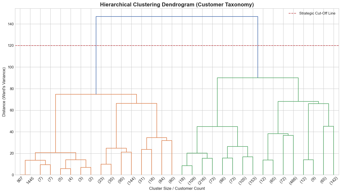
Sub-Segmentation: It reveals relationships between segments. For example, a major branch might represent “High-Value Customers,” which then splits into two smaller sub-branches: “Digital High-Value” and “In-Store High-Value.” This is excellent for creating parent-brand vs. sub-brand marketing architectures.
We will use Ward’s Method, which merges clusters in a way that minimizes the variance within the newly formed clusters, resulting in highly compact and distinct customer personas.
# ==========================================
# Code Cell: Hierarchical Clustering & Dendrogram
# ==========================================
import matplotlib.pyplot as plt
import pandas as pd
from scipy.cluster.hierarchy import dendrogram, linkage
from sklearn.cluster import AgglomerativeClustering

# 1. Create the linkage matrix using Ward's method
# (We continue to use the 'pca_data' generated in Step 4 to avoid high-dimensionality distortion)
linked = linkage(pca_data, method='ward')

# 2. Plot the Dendrogram
plt.figure(figsize=(14, 8))
# We truncate the dendrogram to only show the last few merged levels for readability
dendrogram(linked,
           truncate_mode='level',
           p=4,
           show_leaf_counts=True,
           leaf_rotation=45.,
           leaf_font_size=12.,
           color_threshold=120) # This color threshold visually splits the major branches

plt.title('Hierarchical Clustering Dendrogram (Customer Taxonomy)', fontsize=16, fontweight='bold')
plt.xlabel('Cluster Size / Customer Count')
plt.ylabel('Distance (Ward\'s Variance)')
plt.axhline(y=120, color='r', linestyle='--', label='Strategic Cut-Off Line')
plt.legend()
plt.tight_layout()
plt.show()

# 3. Fit the Agglomerative Model
# Based on looking at the dendrogram branches, we can slice the tree.
# Let's set n_clusters=8 to directly compare these segments against our K-Means model.
hc_model = AgglomerativeClustering(n_clusters=8, metric='euclidean', linkage='ward')
df['Hierarchical_Cluster'] = hc_model.fit_predict(pca_data)

# 4. Managerial Profiling Setup
profiling_features = {
    'Income': 'mean',
    'TotalSpent': 'mean',
    'TotalAccCmp': 'mean',        # Campaign response rate
    'NumWebPurchases': 'mean',    # Digital purchasing behavior
    'Age': 'mean',
    'Recency': 'mean',
    'Complain': 'mean'
}

# 5. Aggregate and combine metrics
hc_profile = df.groupby('Hierarchical_Cluster').agg(profiling_features).round(2)
hc_counts = df['Hierarchical_Cluster'].value_counts().rename('Cluster_Size')
hc_proportions = (df['Hierarchical_Cluster'].value_counts(normalize=True) * 100).round(2).rename('Proportion (%)')
hc_summary = pd.concat([hc_counts, hc_proportions, hc_profile], axis=1).sort_index()

# 6. Apply visual styling (Using Oranges to differentiate from K-Means and DBSCAN)
styled_hc = hc_summary.style.background_gradient(cmap='Oranges') \
                            .format(precision=2) \
                            .highlight_max(color='lightgreen', subset=['Income', 'TotalSpent', 'TotalAccCmp']) \
                            .highlight_max(color='lightcoral', subset=['Recency', 'Complain'])

# 7. Export directly to HTML to bypass Spyder/Console display limitations
with open("hierarchical_cluster_profile.html", "w") as f:
    f.write(styled_hc.to_html())

print("Hierarchical cluster profile successfully generated and saved as 'hierarchical_cluster_profile.html'")
10. Comparing Hierarchical to K-Means#
Once you open the generated HTML file, you will notice that Hierarchical Clustering often identifies similar macroeconomic boundaries (e.g., high-income vs. low-income) as K-Means, but the distribution of the cluster sizes will differ.
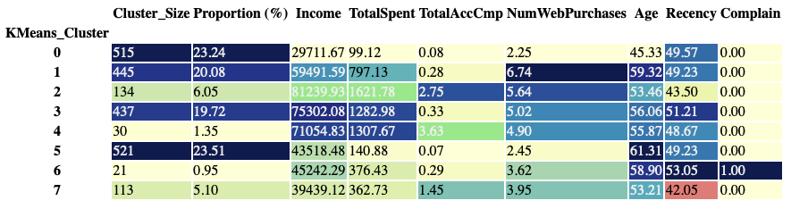
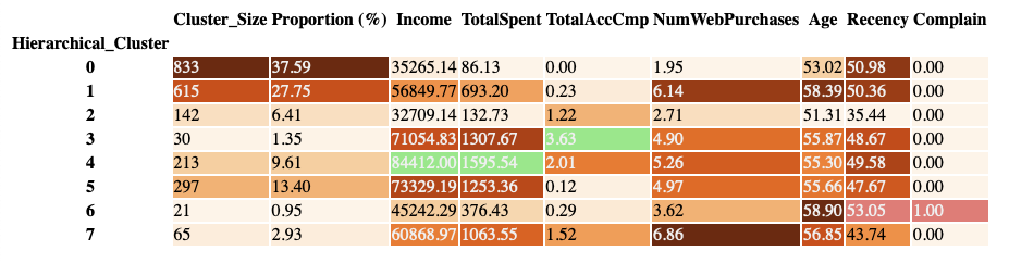
Hierarchical clustering is highly sensitive to the natural variances in the dataset. While K-Means tries to forcefully partition the space into relatively balanced spheres, Ward’s method will happily create a massive parent cluster and several highly specific, niche micro-clusters if that is what the data’s natural variance dictates.
Lecture Takeaway: * Use K-Means when you need \(K\) balanced, operational marketing segments to assign account managers to.
Use Hierarchical when you are conducting deep market research and need to understand the architectural relationship and sub-categories of your entire market.
Use DBSCAN when data integrity is paramount and you need to filter out noise/fraud/outliers before running your campaigns.