Lecture 3: Set, Function, Module, and Pandas

Lecture 3: Set, Function, Module, and Pandas#

In the previous two lectures, we have learned various topics including:

how to work in Spyder IDE to write and compile/interpret Python program,
how to define and manipulate basic Python objects (int, float, bool, string, list, tuples, dictionary, iterable),
how to use basic built-in Python functions and methods (print(), len(), input(), split(), isdigit()),
how to design program flows using branching (if, elif, else) and loops (for, while, list comprehension),
how to define and document custom function and how to do a good defensive programming including how to handle exceptions using the try – except [[– else] – finally] blocks.

In the third lecture we will continue exploring the use of custom function and then move on to discuss modules, which are basically a collection of custom functions, and one fundamental module for data science: Pandas. Before we do that, we will start with one other Python object type which is called set.

Python Set Object#

Defining a set object#

Similar to lists and tupples, we can define a set using the specific notation (curly braces: {}) or the set() constructor function.

With the set constructor, we write:

A = set(<iterables>)

With the curly braces, we need to know the member of the set then define it accordingly:

B = {<obj1>, <obj2>, ...}

For example, let’s considered the word “tomorrow” and we want to construct a set A which members are all the letters which appear in the word “tomorrow”.

s = "tomorrow"
# A is a set of all letters in s
A = set(list(s))
print(A)
print(type(A))

# B is also a set of all letters which appear in the word "tomorrow"
B = {'m', 'w', 'r', 't', 'o'}
print(B)
print(type(B))

{'t', 'w', 'r', 'm', 'o'}
<class 'set'>
{'r', 'm', 't', 'o', 'w'}
<class 'set'>

Some notes about set#

The elements of a set are unordered.
The elements of a set are unique (duplicate elements are not allowed).
A set is mutable; but its elements must be of immutable type. Thus, lists and dictionaries cannot be set elements since they are mutable.

# set elements must be immutable type

# since lists are mutable, they cannot be set element
alist = [1, 2, 3]
myset = {alist}

# since dictionaries are mutable, the cannot be set element
adict = {'a': 1, 'b': 2}
myset = {adict}

---------------------------------------------------------------------------
TypeError                                 Traceback (most recent call last)
Cell In[2], line 5
      1 # set elements must be immutable type
      2 
      3 # since lists are mutable, they cannot be set element
      4 alist = [1, 2, 3]
----> 5 myset = {alist}
      7 # since dictionaries are mutable, the cannot be set element
      8 adict = {'a': 1, 'b': 2}

TypeError: unhashable type: 'list'

We can have an empty set. An empty set can only be defined using the set() function. We cannot use the curly braces notation, such as A = {}, to define A as an empty set.

# empty set can only be defined using set() constructor function.
# this is because empty {} defines a dictionary object
A = set()
print(type(A))
B = {}
print(type(B))

<class 'set'>
<class 'dict'>

The argument to the set() constructor function is an ; it generates a list of elements in the set.
If we define a set using the curly braces notation, then the specified within the curly braces are placed into the set intact, even if they are .

#%% Compare the following two ways to define a set

A = set('tomorrow')
B = {'tomorrow'}

print('This is A:', A)
print('This is B:', B)

#using {}, the whole <iterable> object becomes a set's element 
#using set(), each iterable element becomes a set's element

This is A: {'w', 'r', 't', 'm', 'o'}
This is B: {'tomorrow'}

The set elements can be of different types.

For more details and examples on Python sets, see W3 schools.

Set operator and methods#

Similar to Lists and Tupples, we can use the len() function to count the number of a set’s elements. Operators such as in and not in can also be used to check for a set’s members.

# Operator on a set (e.g., checking set's size and membership)

#The len() function returns the number of elements in a set
A = set('tomorrow')
print('This is A:', A)
print('The object type of A is:', type(A))
print('Number of elements in set A:', len(A))

B = {'tomorrow'}
print('This is B:', B)
print('The object type of B is:', type(B))
print('Number of elements in set B:', len(B))

#The in and not in operators can test for set membership
print("The character 'A' is in the set A.", 'A' in A)
print("The character 'A' is NOT in the set A.", 'A' not in A)
print("The character 'w' is in the set A.", 'w' in A)

print("The character 'w' is NOT in the set B.", 'w' not in B)

This is A: {'w', 'r', 't', 'm', 'o'}
The object type of A is: <class 'set'>
Number of elements in set A: 5
This is B: {'tomorrow'}
The object type of B is: <class 'set'>
Number of elements in set B: 1
The character 'A' is in the set A. False
The character 'A' is NOT in the set A. True
The character 'w' is in the set A. True
The character 'w' is NOT in the set B. True

Union of two sets#

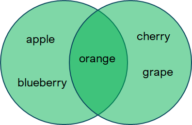
Consider the sets A = {‘apple’, ‘blueberry’, ‘orange’} and B = {‘cherry’, ‘grape’, ‘orange’}. From Math, we know the union of the sets A and B, say \(C = A \cup B\), will have the following elelements {‘apple’, ‘blueberry’, ‘orange, ‘cherry’, ‘grape’}

union

In Python, a union of two sets can be computed using the | operator or the built-in .union() set method.

# Union of sets

# lets have these sets
A = {'apple', 'blueberry', 'orange'}
B = {'cherry', 'orange', 'grape'}

# union of sets is performed using the | operator
C = A|B
print("The object type of C is", type(C))
print(C)

# union of sets can also be performed using .union method
D = A.union(B)
print("The object type of D is", type(D))
print(D)

The object type of C is <class 'set'>
{'cherry', 'apple', 'blueberry', 'grape', 'orange'}
The object type of D is <class 'set'>
{'cherry', 'apple', 'blueberry', 'grape', 'orange'}

Intersection of a set#

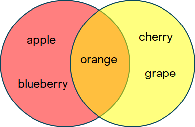
Consider the same sets A = {‘apple’, ‘blueberry’, ‘orange’} and B = {‘cherry’, ‘grape’, ‘orange’} as before. From Math, we know the intersection set \(C = A \cap B = \) {‘orange’}

intersection

In Python, a union of two sets can be computed using the & operator or the built-in .intersection() set method.

# lets have these sets
A = {'apple', 'blueberry', 'orange'}
B = {'cherry', 'orange', 'grape'}

# intersection of sets is found using the & operator
E = A&B
print("The object type of E is", type(E))
print(E)

# intersection of sets is found using .intersection method
F = A.intersection(B)
print("The object type of F is", type(F))
print(F)

The object type of E is <class 'set'>
{'orange'}
The object type of F is <class 'set'>
{'orange'}

Set difference (or relative complement)#

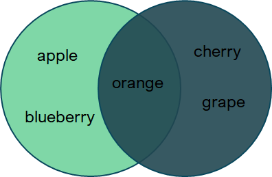
From Math, the difference between two sets A and B is defined as D = A - B in which D contains all elements of A which are not the element of B. (This is why it is also called relative complement).

So, if A and B are as defined above, then D = A - B = {‘apple’, ‘blueberry’}

difference

In Python, the difference between two sets can be computed using the - operator or the built-in .difference() set method.

# Relative complement (i.e. set difference)

# lets have these sets
A = {'apple', 'blueberry', 'orange'}
B = {'cherry', 'orange', 'grape'}

# relative complement of sets is found using the '-' operator
G = A - B
print("The object type of G is", type(G))
print(G)

# relative complement is found using .difference method
H = A.difference(B)
print("The object type of H is", type(H))
print(H)

The object type of G is <class 'set'>
{'apple', 'blueberry'}
The object type of H is <class 'set'>
{'apple', 'blueberry'}

More on Python functions#

How should we write our program#

As a good practice of defensive programming in which we aim to eliminate program bugs, we use functions for program decomposition and abstraction.

Decomposition allows us to split complex and difficult tasks into smaller and easier tasks to be handled by different functions.

Divide the program into modules: break the long (complex code) into simpler pieces. Each module is composed of several
Each module, often consists of functions and classes, is self-contained and can be intended to be reusable
Allow us to better organise our codes and keep them coherent

The abstraction principles suppress details and we only see the relevant input and output. Abstraction allows us to use functions to hide unnecessary complex details and focus on the output of each function that matters for the whole program. Effectively, the abstracted piece of code becomes like a black box.

Defining and calling/invoking a function#

Functions are encapsulated segments of code that perform a set of pre-specified actions. You can use the same function again and again in many different situations. e.g. the print() function. A function can take one or more values as input and return one or more values as output.

A function is defined with the following syntax:

def function_name(argument1, argument2, ...):
    ...
    <code_that_performs_specific_function>
    ...
    return <values_to_return>

Characteristics of a function#

It has a name
It may have parameters
It may have a docstring describing the function
It has a body
It may return something

A simple function definition and call is shown by the following example. Inside the function, we issue a print("inside is_even") to keep track of everytime the function is invoked. As discussed earlier, print() statements could be helpful in debugging to trace the location of possible error in the program.

# function definition
def is_even(i):
    """
        Input: numerical value i.
        Output: return True if i is an even number
    """
    print("inside is_even")
    return i%2==0

# function call
print("3 is even.", is_even(3))
print("6.1 is even.", is_even(6.1))
print("7.5 is even.", is_even(7.5))
print("12 is even.", is_even(12))

inside is_even
3 is even. False
inside is_even
6.1 is even. False
inside is_even
7.5 is even. False
inside is_even
12 is even. True

In the example below, we modified the previous function slightly by introducing a global (i.e. defined outside the function)debugflag variable. Then, the function print(“inside is_even”) statement is only executed conditionally on debugflag==True. This way the real output of interest from the function can be shown without the clutters from the debugging print output.

Note

We could also set the value of debugflag as part of the parameter of the function, such as def is_even(i, debugflag): and then when we invoke the function we use is_even(i=3, debugflag=False) to turn of the print("inside is_even") statement. Can you try to modify the is_even function this way?

#%% Function example: is_even() with conditional debugging print

# debugflag = False
debugflag = True

def is_even(i):
    """
        Input: A numerical value
        Output: return True if i is an even number
    """
    if debugflag:
        print("inside is_even")
    return i%2==0

if debugflag:
    print("outside is_even")
print("3 is even.", is_even(3))

if debugflag:
    print("outside is_even")
print("6.0 is even.", is_even(6.0))

if debugflag:
    print("outside is_even")
print("6.1 is even.", is_even(6.1))

# without debugging clutters
print()
print("Turned off debugging")
debugflag = False
if debugflag:
    print("outside is_even")
print("3 is even.", is_even(3))

if debugflag:
    print("outside is_even")
print("6.0 is even.", is_even(6.0))

if debugflag:
    print("outside is_even")
print("6.1 is even.", is_even(6.1))

outside is_even
inside is_even
3 is even. False
outside is_even
inside is_even
6.0 is even. True
outside is_even
inside is_even
6.1 is even. False

Turned off debugging
3 is even. False
6.0 is even. True
6.1 is even. False

Another example of a simple function: sum_of_squares(). In this example, we write a function which takes two values as inputs and returns the sum of the squared value of the inputs. Later on, we will use this function as a part for applying the Pythagoras theorem pythogoras to compuse the hypotenuse length of a right angle triangle.

def sum_of_squares(x, y):
    """
        Input: two values
        Output: return the sum of the squared input values
    """
    result = x**2 + y**2
    return result

# example of sum_of_squares function call
print(sum_of_squares(2, 5))

# a more informative example using f-string
x = 2
y = 5
print(f"The sum of squares of {x} and {y} is {sum_of_squares(x, y)}")

29
The sum of squares of 2 and 5 is 29

Function output as input to another function#

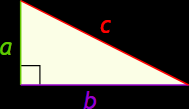
The example below demonstrate one way a function can invoke another function. In this example, the function hypotenuse_length() will return the length of the hypotenuse of a right-angle triangle given the lengths of the triangle’s base and height. Recall, according to the Pythagoras theorem pythagoras, for a right triangle with the lengths of the height = a, base = b, and hypotenuse = c, then \(a^2 + b^2 = c^2\). Thus, if we know the value of \(a\) and \(b\), with a little bit of algebra, we can compute the value of \(c\).

#%% Finding the hypothenuse of a right angle triangle
#Using function output as input to another function)

def sum_of_squares(x, y):
    """
        Input: two values
        Output: return the sum of the squared input values
    """
    result = x**2 + y**2
    return result

def hypotenuse_length(x, y):
    """
        Input: two values representing the height and base length
        Formula: Use Pythoagoras' theorem (c^2 = a^2 + b^2) to calculate the 
        length of the hypotenuse of a right-angle triangle
        Output: return the length of they hypotenuse of right-angle triangle
        for given values of base length and height
    """   
    # Use sum_of_squares() compute (a^2 + b^2) then take its square root 
    result = sum_of_squares(x, y)**0.5     # c is the square-root of the sum of squares
    return result

#Now in the main program
base = 3
height = 4
# Use the output of the hypotenuse_length() function in f-print literal
print(F"The hypotenuse of base={base} & height={height} triangle is",
      F"{hypotenuse_length(base, height)}")  

The hypotenuse of base=3 & height=4 triangle is 5.0

Sepcifying default argument value for a function#

In the next example, we modified our hypotenuse_length function to only take one input value to compute the hypotenuse length of a square right triangle. In this case, base = height, and there is no need to provide the function with two separate but identical input values. In this example, our hypotenuse_length function can polymorph depending on the number of arguments supplied to it. It still “takes” two arguments x and y, but for the second argument if set a default value y = None. That is, if the function is supplied only with one argument, say hypotenuse_length(3), then x is assigned with the value 3, while y is assigned with the value None (which is the default argument value).

Then, within the body of the hypotenuse_length function we have two separate code blocks to deal with whether the right triangle is a square triangle (without y value supplied) or not. In this case, if y is not supplied, we assign y = x to reflect that we are assumming the user of the function is interested in knowing the length of the hypotenuse of a square right triangle.

#%% Function with default argument
def sum_of_squares(x, y):
    """
        Input: two values
        Output: return the sum of the squared input values
    """
    result = x**2 + y**2
    return result

def hypotenuse_length(x, y=None):
    """
        Input: The base [and <height>] of of a right triangle
               If only a single value is supplied, height=base is assumed
        Formula: Use Pythoagoras' theorem (c^2 = a^2 + b^2) to calculate the 
        length of the hypotenuse of a right-angle triangle
        Output: return the length of they hypotenuse of right-angle triangle
        for given values of base length and height
    """   
    
    # If the "y" argument is not passed, assume that y = x
    if y is None:
        y = x
        print(f"base = height = {y}")
    else:
        print(f"base = {x}, height = {y}")
        
    # Use Pythoagoras' theorem (c^2 = a^2 + b^2) to calculate the length of the hypotenuse of a right-angle triangle
    result = sum_of_squares(x, y)**0.5     
    return result

base = 3
height = 4

# now compute the hypotenuse length for a square right triangle with base = height = 3
print(f"The hypotenuse is: {hypotenuse_length(base):.2f}")

# now compute the hypotenuse length for a right triangle with base = 3 and height = 4
print(f"The hypotenuse is: {hypotenuse_length(base, height):.2f}")

base = height = 3
The hypotenuse is: 4.24
base = 3, height = 4
The hypotenuse is: 5.00

The example below shows how to deal with multiple default arguments. In the example, the function hypotenuse_length has three arguments: x, y and print_results. The first argument does not have a default value. The second argument (y) has a default value of None for the case when the triangle for which the length of the hypotenuse is to be computed is a square right triangle in which the base and height have equal values set by the x argument. The third argument (print_results) has a default value of False to turn off all the print statements within the function.

In the example, we see four different ways the function hypotenuse_length is invoked depending on the default values and the ordering of the supplied value to the arguments.

Note

Function arguments are positional, uness you specifically refer to their names

#%% Multiple default arguments, position, and referring by argument names
def hypotenuse_length(x, y=None, print_result=False):
    """
        Input: x = the base of triangle (required argument)
               y = height of triangle (optional, = base if not supplied)
               print_result = boolean flag to print result or not
               
        Formula: Use Pythoagoras' theorem (c^2 = a^2 + b^2) to calculate the 
        length of the hypotenuse of a right-angle triangle
        Output: return the length of they hypotenuse of right-angle triangle
        for given values of base length and height
    """   
    # If the "y" argument is not passed, assume that y = x
    if y is None:
        y = x  
    # Use Pythoagoras' theorem (c^2 = a^2 + b^2) to calculate 
    result = sum_of_squares(x, y)**0.5  
    if print_result is True:
        print(f"Inside function \n hypotenuse = {result:.2f}")
    return result
print("outside function\n", hypotenuse_length(2, print_result=True, y=7))
print("outside function\n",hypotenuse_length(print_result=True, y=7, x=2))
print("outside function\n",hypotenuse_length(2,7,True))
print("outside function\n",hypotenuse_length(2,7))

Inside function 
 hypotenuse = 7.28
outside function
 7.280109889280518
Inside function 
 hypotenuse = 7.28
outside function
 7.280109889280518
Inside function 
 hypotenuse = 7.28
outside function
 7.280109889280518
outside function
 7.280109889280518

Python Modules and Packages#

Modular programming and its benefits#

The use of functions, modules and packages in Python enables us to implement the modular programming approach. In this approach, we break a large, unwieldy programming task into separate, smaller, more manageable subtasks or modules. There are several advantages from doing this including:

Simplicity: a module focuses on one relatively small portion of the problem, making development easier and less error-prone.
Maintainability: Modules can enforce logical boundaries between different problem domains by minimising interdependency to decrease the likelihood that modifications to a single module will have an impact on other parts of the program. This also enable collaborative programming.
Reusability: Functions within a single module can be reused; eliminating the need to duplicate code.
Scoping: Modules separate namespaces to avoid collisions between identifiers in different areas of a program.

Different types of modules and how to use them#

Built-in Pyton modules are those intrinsically contained in the Python interpreters. Examples of these built-in Python modules include the itertools module. More importantly, there are also external modules which are written in Python (for example, the module pandas) and those which are written in C or other languages. These latter modules, such as the regex module, are often faster and can be dynamically loaded by our Python program.

To use and external module (written in either Python or other language), we need to do the following steps:

Install the corresponding package which contains the module (e.g., on PowerShell or Terminal prompt, we issue the command: conda install scipy)
Once the module is installed in our Python environment, we issue the import <module name> statement in our Python program.
- A module may have multiple functions and if we only need to use a specific functions within the module (say to reduce memory load), we can specify it in our import statement as follows: from <module name> import <function names>
- Due to possible long name of the module and its functions, we may assign a shortened object name for the module when we are importing the module. For example: import <module_name> as <alt_name>

A few external modules which are useful for data science and their import statements and common shorthands are listed below:

NumPy (): import numpy as np
Pandas (): import pandas as pd
Matplotlib: import matplotlib.pyplot as plt
SciKit-Learn: import sklearn as sk
BeautifulSoup: import beautifulsoup as bs
StatsModel:
- import statsmodels.api as sm
- from statsmodels.formula.api import ols

PANDAS and DataFrame object#

Pandas is a module for working with data, usually in tabular form. The most important data structure in Pandas is the DataFrame, which we can think of as being similar to an Excel table, or an SQL table.

Let’s import the Pandas module and create a simple DataFrame object using the .DataFrame() method of pandas by supplying data in a literal dictionary object:

import pandas as pd
df = pd.DataFrame({'col_1': [6,7,11], 'col_2': ['a', 'b', 'c']})

In this example, we invoke Pandas’ DataFrame constructor function and set its value to contain two columns, with column headers ‘col_1’ and ‘col_2’ respectively, and three rows. For col_1, the value in each row is int object 6, 7, and 11. For col_2, the value in each row is the string object ‘a’, ‘b’, and ‘c’.

Note

When we created the DataFrame object using Pandas in the above example, there is an automatically created first column which contains the index to the rows of the DataFrame object.

For additional examples not discussed in this note, see W3School-Pandas-Tutorial.

#%% introduction to pandas DataFrame

import pandas as pd

df = pd.DataFrame({'col_1': [6,7,11], 'col_2': ['a', 'b', 'c']})
df

	col_1	col_2
0	6	a
1	7	b
2	11	c

In the example below, we construct a bit more substantial DataFrame object which has a missing value. The missing value is represented by the nan property from the NumPy module. Notice again in this example we supply the values for the row and columns to the DataFrame constructor in the form of a dictionary in which each column:row is presented by the <key>:<value> of the dictionary. In this case, the <key> becomes the column’s heading and the associated <value> is a list of the row elements.

Note

The missing value represented by np.nan is displayed as “NaN” in the DataFrame.

#%% creating a bit more substantial DataFrame

# we import numpy to access its np.nan property to represent missing values
import numpy as np

data = {
    'name': ['Jeff', 'Julia', 'Ronda', 'Dinesh', 'Susan'],
    'height': [183, 176, 187, 157, 162],
    'weight': [69, 73, np.nan, 77, 82],
    'gender': ['m', 'f', 'f', 'm', 'f']
}

df = pd.DataFrame(data)

# we import display method from IPython to use the command noninteractively (i.e. without having to use the IP prompt)
from IPython.display import display

display(df)

	name	height	weight	gender
0	Jeff	183	69.0	m
1	Julia	176	73.0	f
2	Ronda	187	NaN	f
3	Dinesh	157	77.0	m
4	Susan	162	82.0	f

Pandas Series Object#

A pandas’ Series object is similar to a single column in a worksheet such as Excel. To create a pandas’ Series object, we use the pandas .Series() constructor method :

s = pd.Series([39, 43, 25])
print(s)

If we select a specific column in a DataFrame object, we will get a Series object. That is, each column in a Pandas DataFrame is called Pandas Series Object. The example below shows how we can select a single column or a single Pandas Series object.

#%% Selecting a single column from a DataFrame
import numpy as np

data = {
    'name': ['Jeff', 'Julia', 'Ronda', 'Dinesh', 'Susan'],
    'height': [183, 176, 187, 157, 162],
    'weight': [69, 73, np.nan, 77, 82],
    'gender': ['m', 'f', 'f', 'm', 'f']
}

df = pd.DataFrame(data)
display(df)

s = df['name']
print(f"The object type of s is: {type(s)}")

display(s)

	name	height	weight	gender
0	Jeff	183	69.0	m
1	Julia	176	73.0	f
2	Ronda	187	NaN	f
3	Dinesh	157	77.0	m
4	Susan	162	82.0	f

The object type of s is: <class 'pandas.core.series.Series'>

    Jeff
   Julia
   Ronda
  Dinesh
   Susan
Name: name, dtype: object

The following example shows how to select multiple columns from a DataFrame. In this case, the new object containing a subset of a given DataFrame’s columns will also be a DataFrame.

#%% Selecting multiple columns from a DataFrame
import numpy as np

data = {
    'name': ['Jeff', 'Julia', 'Ronda', 'Dinesh', 'Susan'],
    'height': [183, 176, 187, 157, 162],
    'weight': [69, 73, np.nan, 77, 82],
    'gender': ['m', 'f', 'f', 'm', 'f']
}

df = pd.DataFrame(data)
display(df)

s = df[['name','height']]
print(f"The object type of s is: {type(s)}")

display(s)

	name	height	weight	gender
0	Jeff	183	69.0	m
1	Julia	176	73.0	f
2	Ronda	187	NaN	f
3	Dinesh	157	77.0	m
4	Susan	162	82.0	f

The object type of s is: <class 'pandas.core.frame.DataFrame'>

	name	height
0	Jeff	183
1	Julia	176
2	Ronda	187
3	Dinesh	157
4	Susan	162

Selecting rows of a DataFrame#

The syntax to select rows of a DataFrame object named df is as follows: df[<condition>] or df.loc[<condition>]. The <condition> can be multiple conditions which are enclosed in parantheses. For these multiple conditons, we may use the element-wise logical operators & for and and | for or.

# example for selecting DataFrame rows

data = {
    'name': ['Jeff', 'Julia', 'Ronda', 'Dinesh', 'Susan'],
    'height': [183, 176, 187, 157, 162],
    'weight': [69, 73, np.nan, 77, 82],
    'gender': ['m', 'f', 'f', 'm', 'f']
}

df = pd.DataFrame(data)
display(df)

# selecting row with name equals 'Julia'
display(df.loc[df['name'] == 'Julia'])
display(df[df['name'] == 'Julia'])

# selecting rows with 'f' as gender
display(df[df['gender'] == 'f'])

# selecting rowth with names other than 'Ronda
display(df[df['name'] != 'Ronda'])

# Multiple conditions
df[(df['gender'] == 'f') | (df['height'] > 180)]

#%% Some manipulation of pandas' column (i.e. Series)

data = {
    'name': ['Jeff', 'Julia', 'Ronda', 'Dinesh', 'Susan'],
    'height': [183, 176, 187, 157, 162],
    'weight': [69, 73, np.nan, 77, 82],
    'gender': ['m', 'f', 'f', 'm', 'f']
}

df = pd.DataFrame(data)
display(df)

	name	height	weight	gender
0	Jeff	183	69.0	m
1	Julia	176	73.0	f
2	Ronda	187	NaN	f
3	Dinesh	157	77.0	m
4	Susan	162	82.0	f

	name	height	weight	gender
1	Julia	176	73.0	f

	name	height	weight	gender
1	Julia	176	73.0	f

	name	height	weight	gender
1	Julia	176	73.0	f
2	Ronda	187	NaN	f
4	Susan	162	82.0	f

	name	height	weight	gender
0	Jeff	183	69.0	m
1	Julia	176	73.0	f
3	Dinesh	157	77.0	m
4	Susan	162	82.0	f

	name	height	weight	gender
0	Jeff	183	69.0	m
1	Julia	176	73.0	f
2	Ronda	187	NaN	f
3	Dinesh	157	77.0	m
4	Susan	162	82.0	f

Some usefule DataFrame attributes & methods#

.info() provides information on column names, numbers of non-missing values and data types of each column
.columns() provides column names, which can be cast to a list of column names
.unique() is a Series method which gives the unique values in a DataFrame column
describe() is a DataFrame method which provides simple descriptive statistics for each column with numeric or object data type. The descriptive statistics included are:
- count: count of the number of non-NA/null observations,
- mean: mean of the values,
- std: standard deviation of the observations,
- min: minimum of the values,
- max: maximum of the values,
- the 25th, 50th (median), and 75th percentiles.

For many more attributes and methods of pandas DataFrame, see pandas.

#%% Some usefule DataFrame attributes & methods

# we will use the 'iris' data set which comes with the module seaborn
import seaborn as sns

# get the 'iris' data into a DataFrame 'irisdf'
irisdf = sns.load_dataset('iris')

# get info on colum names, non-missing values and datatypes
irisdf.info()

#df.columns provides column names, which can be cast to a list of column names
colnames = list(irisdf.columns)
print("Column names:", colnames)

#.unique() is a Series method which gives the unique values in a DataFrame column
print(irisdf['species'])
uniquespecies = list(irisdf['species'].unique())
print("Unique species: ", uniquespecies)

# .describe() is a DataFrame method which provides simple descriptive statistics 
irisdf.describe()

<class 'pandas.core.frame.DataFrame'>
RangeIndex: 150 entries, 0 to 149
Data columns (total 5 columns):
 #   Column        Non-Null Count  Dtype  
---  ------        --------------  -----  
 0   sepal_length  150 non-null    float64
 1   sepal_width   150 non-null    float64
 2   petal_length  150 non-null    float64
 3   petal_width   150 non-null    float64
 4   species       150 non-null    object 
dtypes: float64(4), object(1)
memory usage: 6.0+ KB
Column names: ['sepal_length', 'sepal_width', 'petal_length', 'petal_width', 'species']
0         setosa
1         setosa
2         setosa
3         setosa
4         setosa
         ...    
145    virginica
146    virginica
147    virginica
148    virginica
149    virginica
Name: species, Length: 150, dtype: object
Unique species:  ['setosa', 'versicolor', 'virginica']

	sepal_length	sepal_width	petal_length	petal_width
count	150.000000	150.000000	150.000000	150.000000
mean	5.843333	3.057333	3.758000	1.199333
std	0.828066	0.435866	1.765298	0.762238
min	4.300000	2.000000	1.000000	0.100000
25%	5.100000	2.800000	1.600000	0.300000
50%	5.800000	3.000000	4.350000	1.300000
75%	6.400000	3.300000	5.100000	1.800000
max	7.900000	4.400000	6.900000	2.500000

Saving/Loading DataFrame to/from files#

Saving to CSV (comma separated) text file: : df.to_csv(<filename>, index=False). Note: the index=False argument is so that the DataFrame index is not save as a new unnamed column in the CSV file.
Loading from CSV (comma separated) text file: df = pd.read_csv(<filename>)
Saving to Excel file: df.to_excel(<filename>)
Loading from CSV (comma separated) text file: df = pd.read_excel(<filename>)

#%% Saving and loading DataFrame to/from a comma separated (csv) file
data = {
    'name': ['Jeff', 'Julia', 'Ronda', 'Dinesh', 'Susan'],
    'height': [183, 176, 187, 157, 162],
    'weight': [69, 73, np.nan, 77, 82],
    'gender': ['m', 'f', 'f', 'm', 'f']
}

df = pd.DataFrame(data)
display(df)
df.to_csv('mydataframe.csv')
df.to_csv('mydataframe2.csv', index=False)
df2 = pd.read_csv('mydataframe.csv')
display(df2)
df3 = pd.read_csv('mydataframe2.csv')
display(df3)

	name	height	weight	gender
0	Jeff	183	69.0	m
1	Julia	176	73.0	f
2	Ronda	187	NaN	f
3	Dinesh	157	77.0	m
4	Susan	162	82.0	f

	Unnamed: 0	name	height	weight	gender
0	0	Jeff	183	69.0	m
1	1	Julia	176	73.0	f
2	2	Ronda	187	NaN	f
3	3	Dinesh	157	77.0	m
4	4	Susan	162	82.0	f

	name	height	weight	gender
0	Jeff	183	69.0	m
1	Julia	176	73.0	f
2	Ronda	187	NaN	f
3	Dinesh	157	77.0	m
4	Susan	162	82.0	f

Slicing DataFrame#

We can select specific (rows, columns) of the DataFrame using slicing with .loc and .iloc as shown in the following examples.

#%% slicing DataFrame
df = pd.read_csv('mydataframe2.csv')
display(df)

# Selecting from Row 2, and the "height" column
display(df.loc[2, 'height'])

# Selecting all rows from 1 to 3, and the "height" column
display(df.loc[1:3, 'height'])

# Select from Row 2 until the last row, all columns
display(df.loc[2:])

display(df[['name', 'weight']])

	name	height	weight	gender
0	Jeff	183	69.0	m
1	Julia	176	73.0	f
2	Ronda	187	NaN	f
3	Dinesh	157	77.0	m
4	Susan	162	82.0	f

  176
  187
  157
Name: height, dtype: int64

	name	height	weight	gender
2	Ronda	187	NaN	f
3	Dinesh	157	77.0	m
4	Susan	162	82.0	f

	name	weight
0	Jeff	69.0
1	Julia	73.0
2	Ronda	NaN
3	Dinesh	77.0
4	Susan	82.0

Adding and renaming column#

To add a column to a DataFramew, we simply assign a new column name of the DataFrame with a list of values which represent the corresponding row values. To rename a column of a DataFrame, we simply use the .rename() method and supply it with a dictionary {:}.

These can be done as shown in the examples below.

# adding column
df = pd.read_csv('mydataframe.csv')
display(df)

df['age'] = [39, 43, 25, 68, 20]
display(df)

df['last_name'] = ['Smith', 'Gulia', 'Berchmore', 'Jayasurya', 'Sarandon']
display(df)


# renaming column
df = df.rename(columns={'name': 'first_name',
                   'height': 'height (cm)',
                   'weight': 'weight (kg)'})

display(df)

	Unnamed: 0	name	height	weight	gender
0	0	Jeff	183	69.0	m
1	1	Julia	176	73.0	f
2	2	Ronda	187	NaN	f
3	3	Dinesh	157	77.0	m
4	4	Susan	162	82.0	f

	Unnamed: 0	name	height	weight	gender	age
0	0	Jeff	183	69.0	m	39
1	1	Julia	176	73.0	f	43
2	2	Ronda	187	NaN	f	25
3	3	Dinesh	157	77.0	m	68
4	4	Susan	162	82.0	f	20

	Unnamed: 0	name	height	weight	gender	age	last_name
0	0	Jeff	183	69.0	m	39	Smith
1	1	Julia	176	73.0	f	43	Gulia
2	2	Ronda	187	NaN	f	25	Berchmore
3	3	Dinesh	157	77.0	m	68	Jayasurya
4	4	Susan	162	82.0	f	20	Sarandon

	Unnamed: 0	first_name	height (cm)	weight (kg)	gender	age	last_name
0	0	Jeff	183	69.0	m	39	Smith
1	1	Julia	176	73.0	f	43	Gulia
2	2	Ronda	187	NaN	f	25	Berchmore
3	3	Dinesh	157	77.0	m	68	Jayasurya
4	4	Susan	162	82.0	f	20	Sarandon

Creating column using existing columns#

This is done by assigning a new column with the existing column or a statement based on transformation of the existing column(s) as shown in the example below.

#%% creating new column based on other columns
df = pd.read_csv('mydataframe.csv')
display(df)
df['last_name'] = ['Smith', 'Gulia', 'Berchmore', 'Jayasurya', 'Sarandon']
df = df.rename(columns={'name': 'first_name',
                   'height': 'height (cm)',
                   'weight': 'weight (kg)'})
df['full_name'] = df['first_name'] + ' '+ df['last_name']
display(df['full_name'])
display(df)

	Unnamed: 0	name	height	weight	gender
0	0	Jeff	183	69.0	m
1	1	Julia	176	73.0	f
2	2	Ronda	187	NaN	f
3	3	Dinesh	157	77.0	m
4	4	Susan	162	82.0	f

        Jeff Smith
       Julia Gulia
   Ronda Berchmore
  Dinesh Jayasurya
    Susan Sarandon
Name: full_name, dtype: object

	Unnamed: 0	first_name	height (cm)	weight (kg)	gender	last_name	full_name
0	0	Jeff	183	69.0	m	Smith	Jeff Smith
1	1	Julia	176	73.0	f	Gulia	Julia Gulia
2	2	Ronda	187	NaN	f	Berchmore	Ronda Berchmore
3	3	Dinesh	157	77.0	m	Jayasurya	Dinesh Jayasurya
4	4	Susan	162	82.0	f	Sarandon	Susan Sarandon

Using the .apply() method#

For example, if we want to count the fullname’s length, we can use the .apply() method on the full_name column to apply the len() built in method of a string object. Then, we can store the computed length in new column 'full_name_len'.

df = pd.read_csv('mydataframe.csv')
display(df)
df['last_name'] = ['Smith', 'Gulia', 'Berchmore', 'Jayasurya', 'Sarandon']
df = df.rename(columns={'name': 'first_name',
                   'height': 'height (cm)',
                   'weight': 'weight (kg)'})
df['full_name'] = df['first_name'] + ' '+ df['last_name']
display(df['full_name'])
display(df)

# Create new column containing number of characters in each person's full_name
df['full_name_len'] = df['full_name'].apply(len)
display(df[['full_name_len', 'full_name']])

	Unnamed: 0	name	height	weight	gender
0	0	Jeff	183	69.0	m
1	1	Julia	176	73.0	f
2	2	Ronda	187	NaN	f
3	3	Dinesh	157	77.0	m
4	4	Susan	162	82.0	f

        Jeff Smith
       Julia Gulia
   Ronda Berchmore
  Dinesh Jayasurya
    Susan Sarandon
Name: full_name, dtype: object

	Unnamed: 0	first_name	height (cm)	weight (kg)	gender	last_name	full_name
0	0	Jeff	183	69.0	m	Smith	Jeff Smith
1	1	Julia	176	73.0	f	Gulia	Julia Gulia
2	2	Ronda	187	NaN	f	Berchmore	Ronda Berchmore
3	3	Dinesh	157	77.0	m	Jayasurya	Dinesh Jayasurya
4	4	Susan	162	82.0	f	Sarandon	Susan Sarandon

	full_name_len	full_name
0	10	Jeff Smith
1	11	Julia Gulia
2	15	Ronda Berchmore
3	16	Dinesh Jayasurya
4	14	Susan Sarandon

Merging DataFrames#

The basic syntax to merge DataFrames is newmergedf = pd.merge(<leftdataframe>, <rightdataframe>, on='<mergecolumnname>', how='left'|'inner'|'right'|'outer') For merging on different column names: newmergedf = pd.merge(<leftdataframe>, <rightdataframe>, left_on='<leftdataframecolumnname>', right_on='<rightdataframecolumnname>', 'how='left'|'inner'|'right'|'outer')

Given two DataFrames zoo and zoo_eats we can conduct four types of merge as shown below: inner, outer, left, and right. These four types of merge is defined by the value we assign to the argument how=:

how='left' gives us the left merge.
how='inner' gives us the inner merge
how='outer' gives us the outer merge
how='right' gives us the right merge.

merging

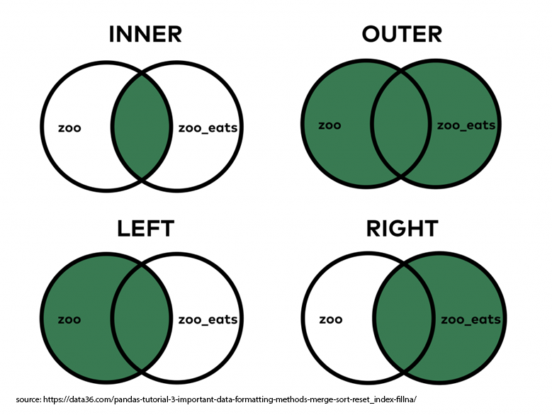
The following examples illustrate how to execute these merge.

Note

The default merge type as set by the argument how= is `left’.

income = pd.read_csv('income.csv')
df = pd.read_csv('mydataframe.csv')
df = df.rename(columns={'name': 'first_name',
                   'height': 'height (cm)',
                   'weight': 'weight (kg)'})

# This joins "df" to "income" by matching the "first_name" column
merged = pd.merge(df, income, on='first_name')
print(merged)

#Note that only the two people that are present in both df and income 
#appear in the resulting merged dataframe. This is because the default 
#join type in pd.merge() is an INNER join.

#LEFT join
merged = pd.merge(df, income, on='first_name', how='left')
display(merged)

#%% Merging on different column names

phd = pd.read_csv('phd.csv')
display(phd)

all_data = pd.merge(merged, phd, left_on='first_name', right_on='name', how='left')
display(all_data[['name','first_name','phd']])

   Unnamed: 0 first_name  height (cm)  weight (kg) gender  income
0           1      Julia          176         73.0      f   19000
1           3     Dinesh          157         77.0      m   56000

	Unnamed: 0	first_name	height (cm)	weight (kg)	gender	income
0	0	Jeff	183	69.0	m	NaN
1	1	Julia	176	73.0	f	19000.0
2	2	Ronda	187	NaN	f	NaN
3	3	Dinesh	157	77.0	m	56000.0
4	4	Susan	162	82.0	f	NaN

	name	phd	phd_year
0	Jeff	False	NaN
1	Julia	True	2015.0
2	Susan	False	NaN

	name	first_name	phd
0	Jeff	Jeff	False
1	Julia	Julia	True
2	NaN	Ronda	NaN
3	NaN	Dinesh	NaN
4	Susan	Susan	False

Lecture 3: Set, Function, Module, and Pandas

Contents

Lecture 3: Set, Function, Module, and Pandas#

Python Set Object#

Defining a set object#

Some notes about set#

Set operator and methods#

Union of two sets#

Intersection of a set#

Set difference (or relative complement)#

More on Python functions#

How should we write our program#

Defining and calling/invoking a function#

Characteristics of a function#

Function output as input to another function#

Sepcifying default argument value for a function#

Python Modules and Packages#

Modular programming and its benefits#

Different types of modules and how to use them#

PANDAS and DataFrame object#

Pandas Series Object#

Selecting rows of a DataFrame#

Some usefule DataFrame attributes & methods#

Saving/Loading DataFrame to/from files#

Slicing DataFrame#

Adding and renaming column#

Creating column using existing columns#

Using the .apply() method#

Merging DataFrames#